Difference between revisions of "Offline Monitoring Data Validation PrimEx"
(→TOF) |
(→TOF) |
||
| Line 614: | Line 614: | ||
<html> | <html> | ||
| − | Occupancy plot: look for "gaps" indicative of missing counters | + | *Occupancy plot: look for "gaps" indicative of missing counters |
| − | Matching TOF Hits: X and Y (right most plots) distributions should be centered close to zero (vertical) | + | *Matching TOF Hits: X and Y (right most plots) distributions should be centered close to zero (vertical) |
| + | *TOF mathching in 1d histograms should have regions larger than 80% | ||
</html> | </html> | ||
Revision as of 09:18, 26 January 2024
This page contains the procedure for checking if PrimEx-η production runs are of good quality and can be used for physics analysis. This page is a work in progress and should not (yet) be used as a reference
Contents
Run Periods
- RunPeriod-2019-01 Validation (PrimEx-η Phase I)
- RunPeriod-2021-08 Validation (PrimEx-η Phase II)
- RunPeriod-2022-08 Validation (PrimEx-η Phase III)
Procedure
For each production run, do the following:
- Go to the Offline Run Browser page.
- Follow the steps outlined in the checklist below.
- Workers should check each plot for their assigned subsystem and leave notes in the corresponding spreadsheet if any significant deviations are seen
- On the spreadsheet, enter "Y" in the "Overall Quality" field if all monitoring histograms are acceptable, otherwise enter "N"
- We will iterate this procedure until the process converges
Expert Actions
- Certify that each subsystem is okay
- Set run status in RCDB based on monitoring results
- (script provided)
Run Statuses
- -1 - unchecked
- 0 - rejected (not physics-quality)
- 1 - approved
- 2 - approved long/"mode 8" data
- 3 - calibration / systematic studies
Checklist
Example Monitoring Spreadsheet (template, incomplete)
General Notes
- Reference runs are listed for each target type
- Be Empty: 110453 (left out of monitoring launches 01-11)
- Be Full: 110551
- He Empty: 111917
- He Full: 111884
TEMP: To Do
Experts should update the table as tasks are completed
| Subdetector | Plots | Instructions | Expert(s) |
|---|---|---|---|
| BCAL | Confirm existing ones are relevant | Confirm existing ones are accurate | Mark Dalton, Zisis Papandreou, Igal Jaegle |
| CCAL | Select relevant plots | Write instructions for volunteers | Drew Smith |
| CDC | Good | Good | Naomi Jarvis |
| FCAL | Confirm existing ones are relevant | Write instructions for volunteers | Mark Dalton, Malte Albrecht, Igal Jaegle |
| FDC | Confirm existing ones are relevant | Write instructions for volunteers | Lubomir Pentchev |
| PS | Confirm existing ones are relevant | Confirm existing ones are accurate | Alex Somov, Olga Cortes |
| SC | Confirm existing ones are relevant | Write instructions for volunteers | Beni Zihlmann |
| TAGH | Confirm existing ones are relevant | Confirm existing ones are accurate | Alex Somov, Bo Yu |
| TAGM | Confirm existing ones are relevant | Confirm existing ones are accurate | Richard Jones, Ellie Prather |
| TOF | Confirm existing ones are relevant | Write instructions for volunteers | Paul Eugenio, Beni Zihlmann |
| RF | Good | Good | Sean Dobbs, Beni Zihlmann |
| Timing | Good | Good | Sean Dobbs |
| Analysis | Confirm existing ones are relevant | Confirm existing ones are accurate | Alex Austregesilo, Sean Dobbs |
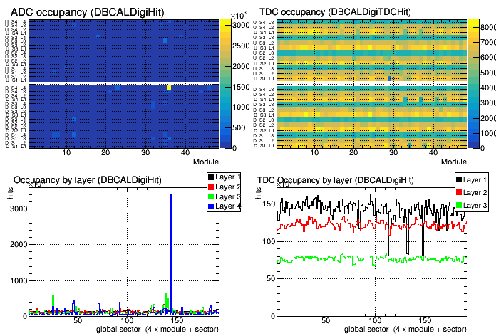
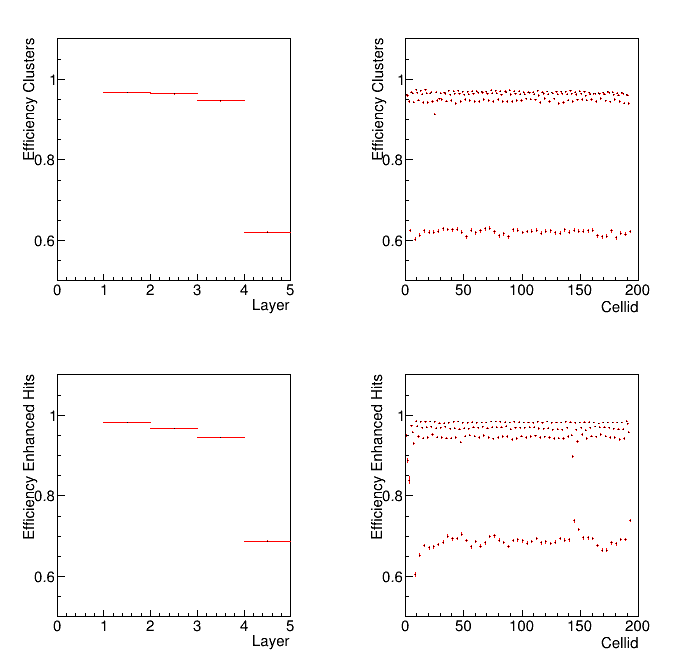
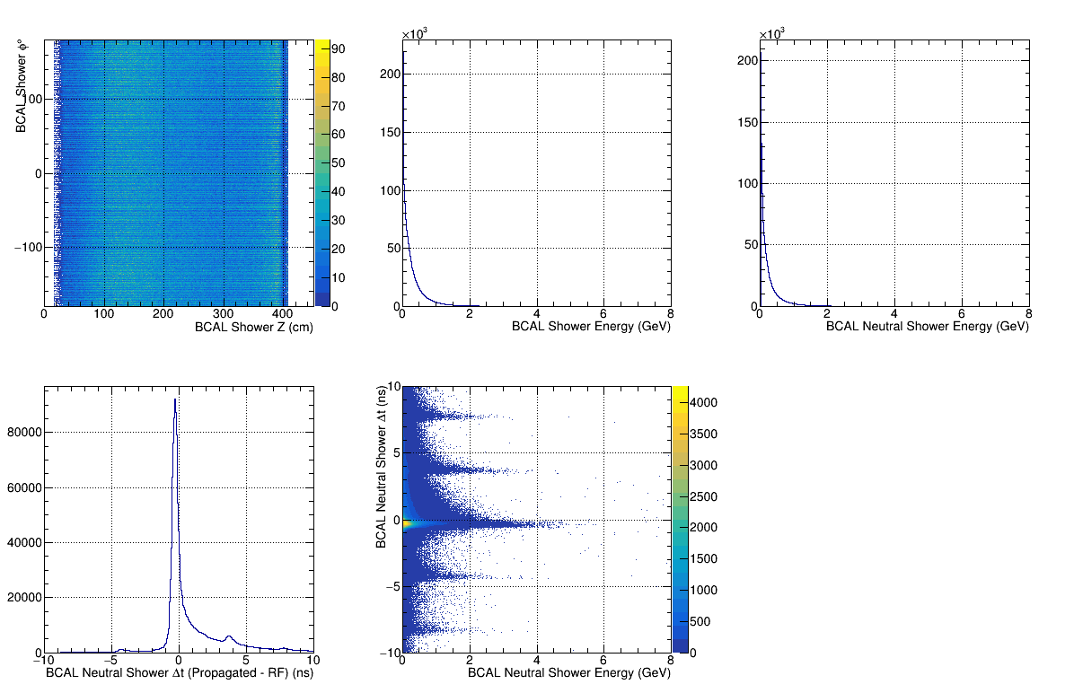
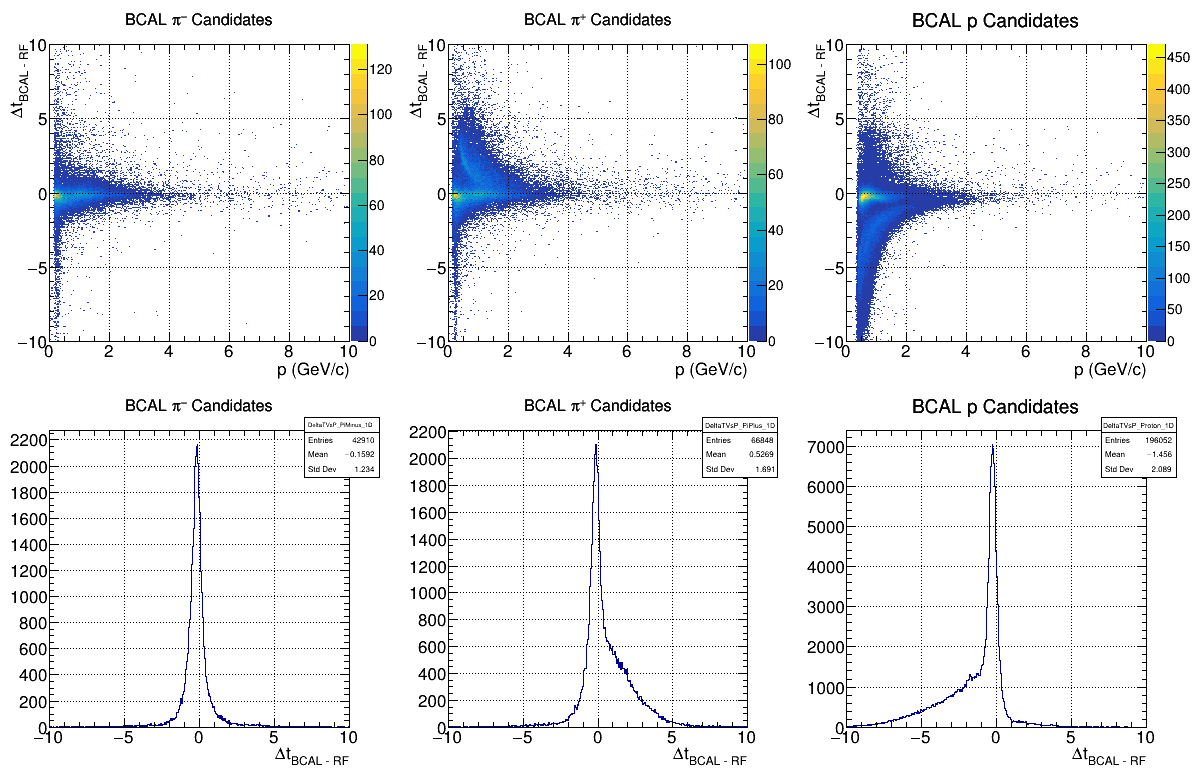
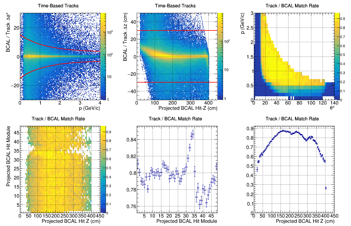
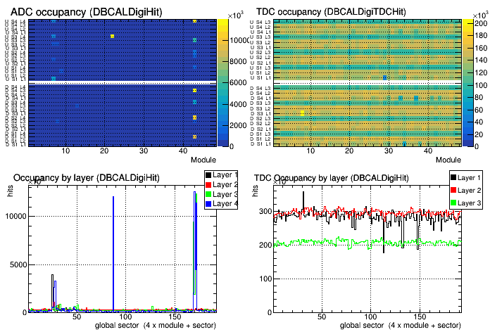
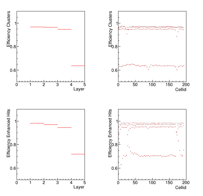
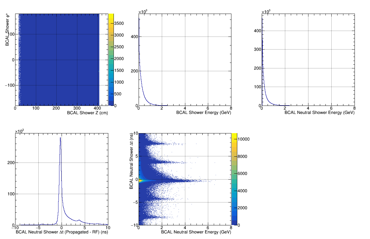
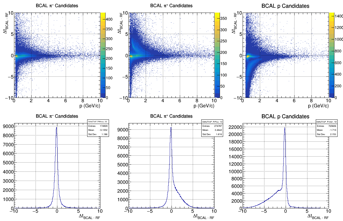
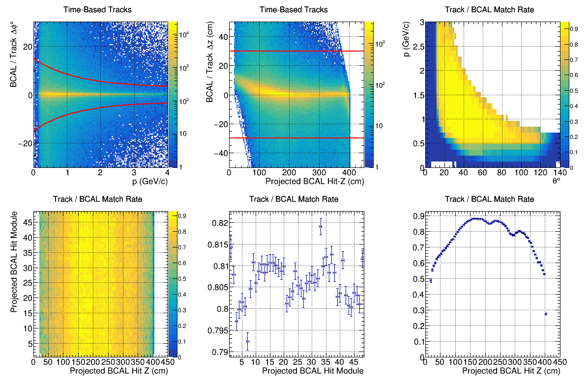
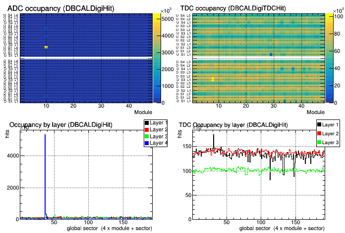
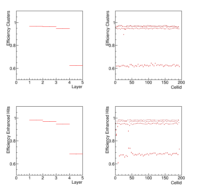
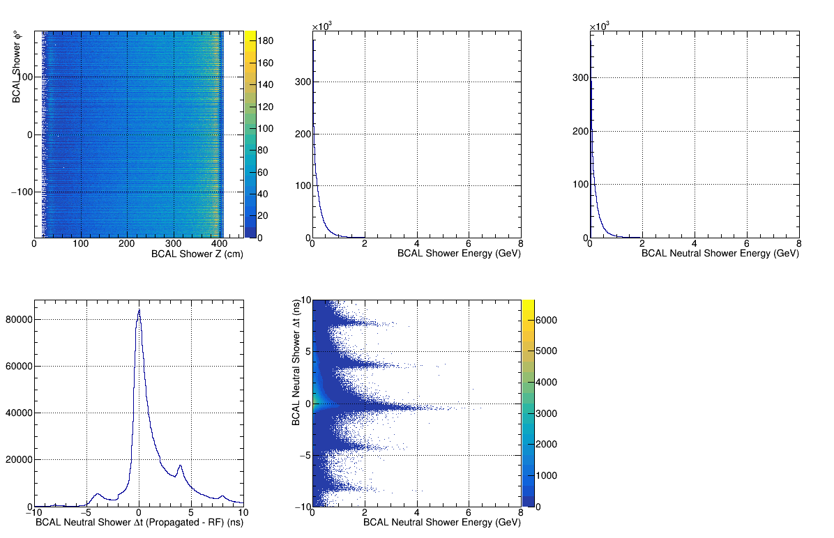
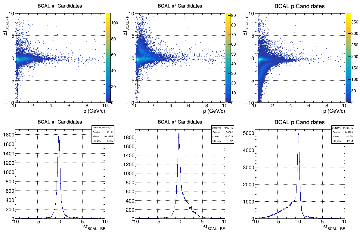
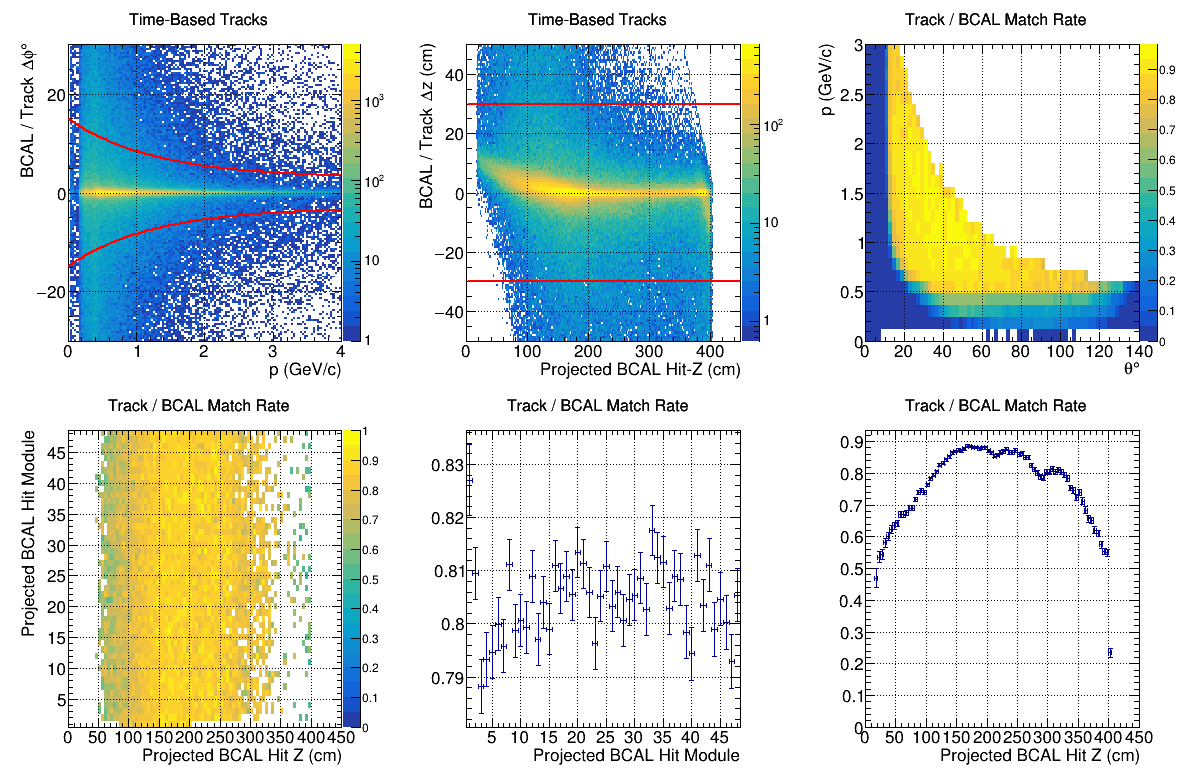
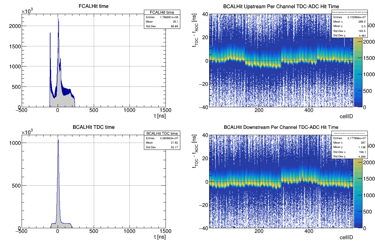
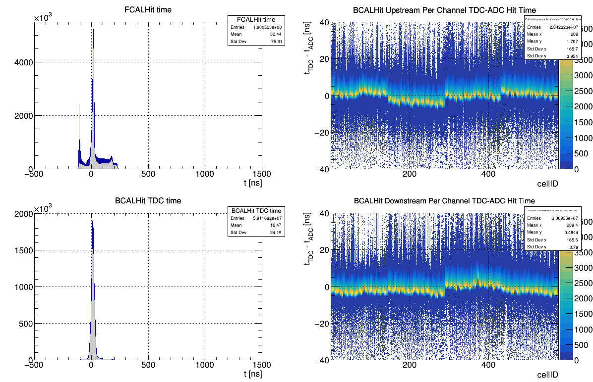
BCAL
- Check Occupancy - Reference: [ link ]
- Check Hit Efficiency - Reference: [ link ]
- Check Recon. BCAL 1 - Reference: [ link ]
- Check Recon. BCAL 2 - Reference: [ link ]
- Check BCAL Matching - Reference: [ link ]
BCAL Reference Plots
Beryllium Target


Full Liquid Helium Target
Empty Liquid Helium Target
BCAL Notes
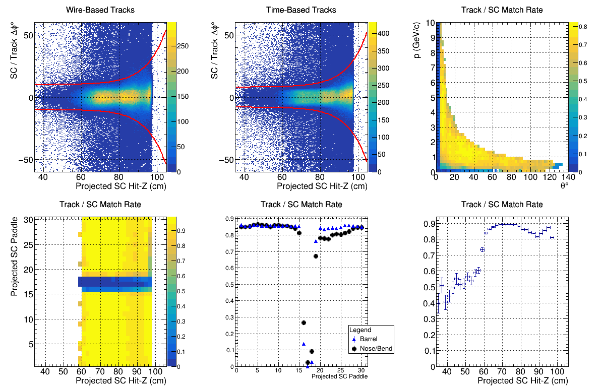
The BCAL is used to measure the energy and time of showers.
The energy is vital for the neutrals. But it’s also used for charged particles to do PID.
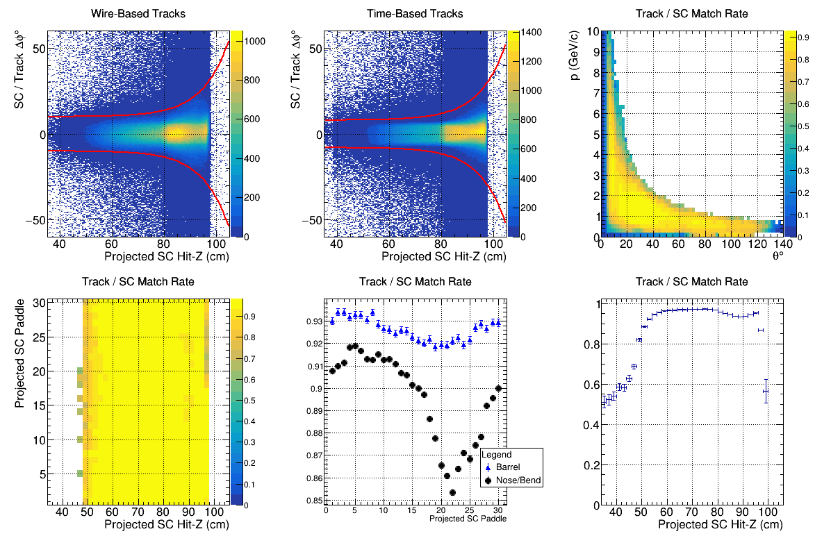
BCAL Matching: These plots are for charged particles that are tracked in the drift chambers and projected to the BCAL. The z position along the BCAL can be calculated using the time difference between upstream and downstream hits and compared to the extrapolated position using the drift chambers.
BCAL/Track Delta z = (z determined from time of up - down hits in BCAL) - (z determined from the extrapolation of tracks in the drift chambers)
projected BCAL Hit-Z = z determined by extrapolating tracks in the drift chambers to the BCAL.
The match rate is the ratio of (number of hits in the BCAL that match the extrapolation of tracks in the drift chamber) / (number of tracks in the drift chamber that point at the BCAL).
CCAL
- List of plots to check goes here
CCAL Reference Plots
Beryllium Target
links to CCAL plots go here
Full Liquid Helium Target
links to CCAL plots go here
Empty Liquid Helium Target
links to CCAL plots go here
CCAL Notes
Instructions for monitoring volunteers go here.
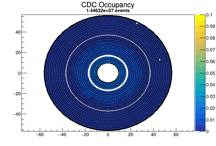
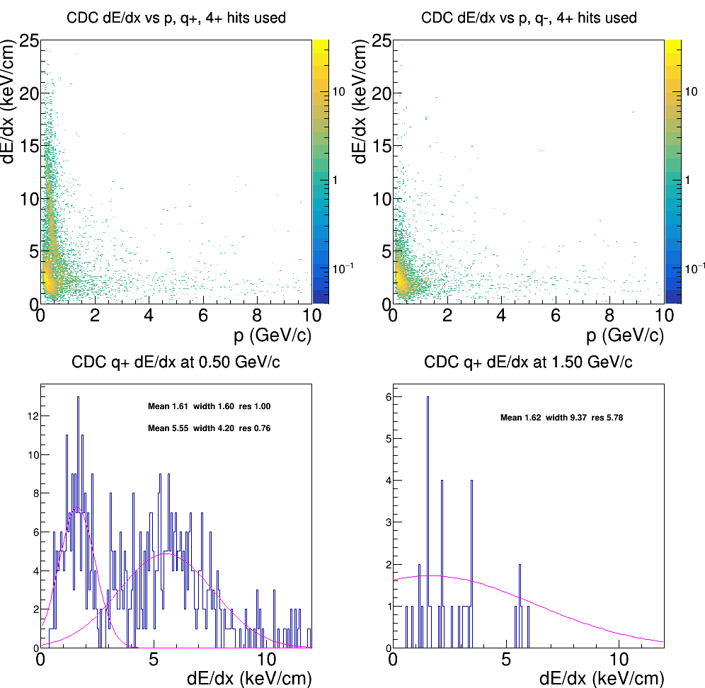
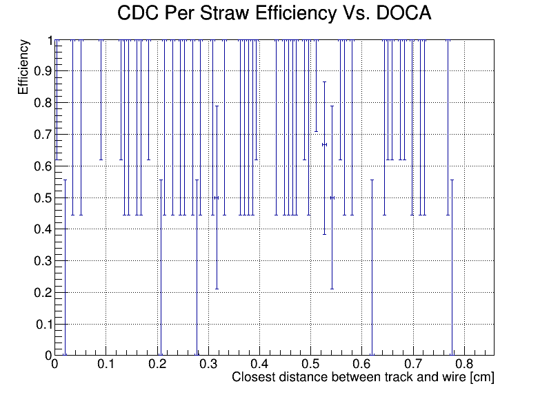
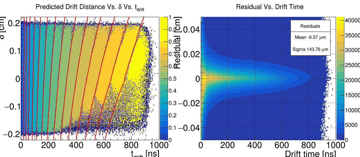
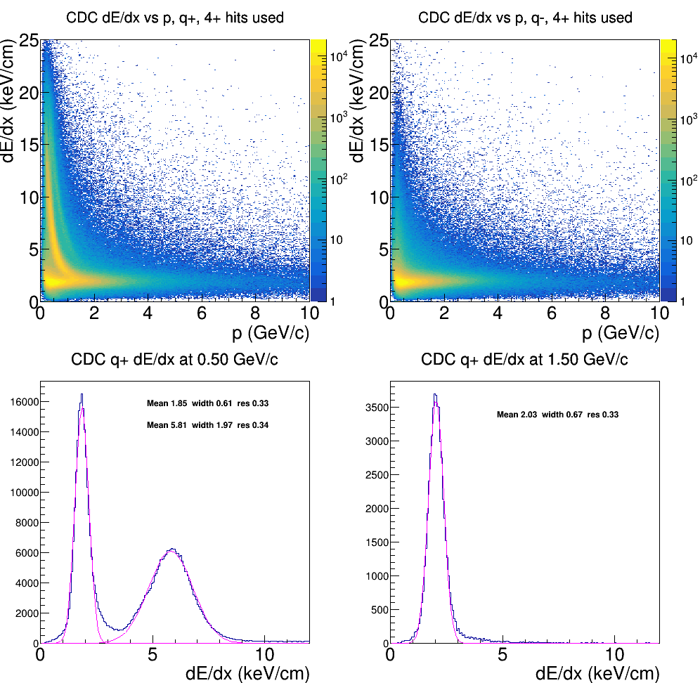
CDC
- Check Occupancy - Reference: [ link ]
- Check Time-to-distance - Reference: [ link ]
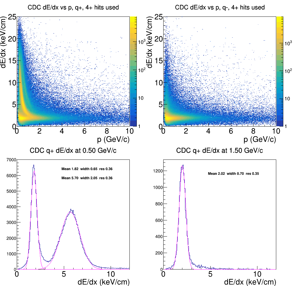
- Check dE/dx - Reference: [ link ]
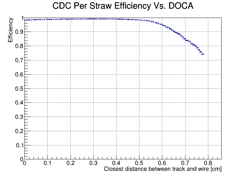
- Check Efficiency - Reference: [ link ]
CDC Reference Plots
Beryllium Target


Absent Beryllium Target

Full Liquid Helium Target

Empty Liquid Helium Target


CDC Notes
General notes on empty/absent Be target runs: the statistics are really low. Mark these runs good unless there is something odd or bad that isn't due to lack of statistics.
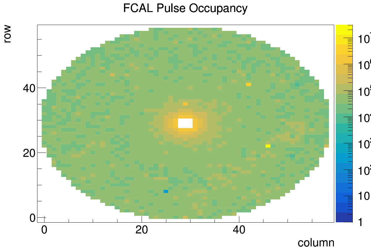
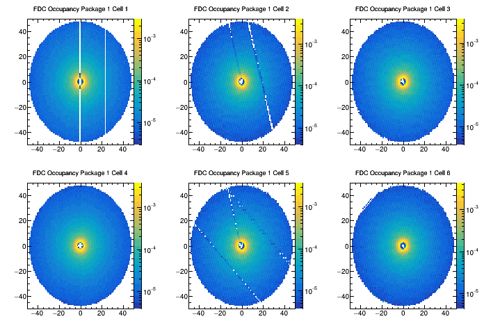
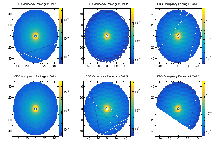
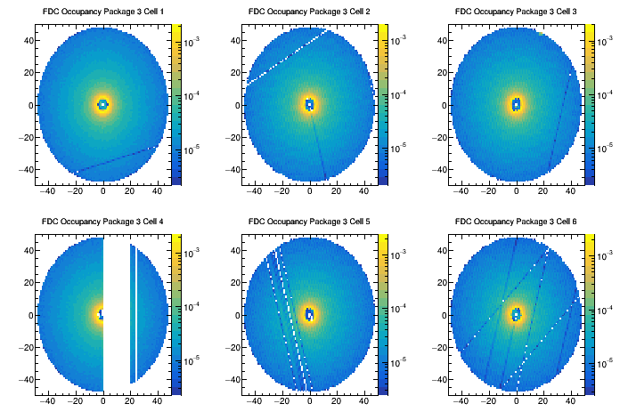
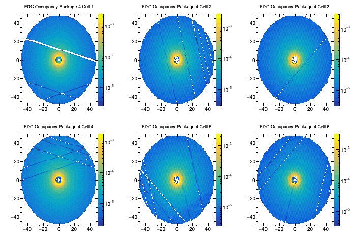
CDC Occupancy: There should be a uniform decrease in intensity from the center of the detector outward. Random white cells scattered throughout occur when not enough data were collected, eg empty target runs, trigger tests or no beam. Several contiguous white, dark blue or bright yellow cells which don't match the neighboring cells are a problem.
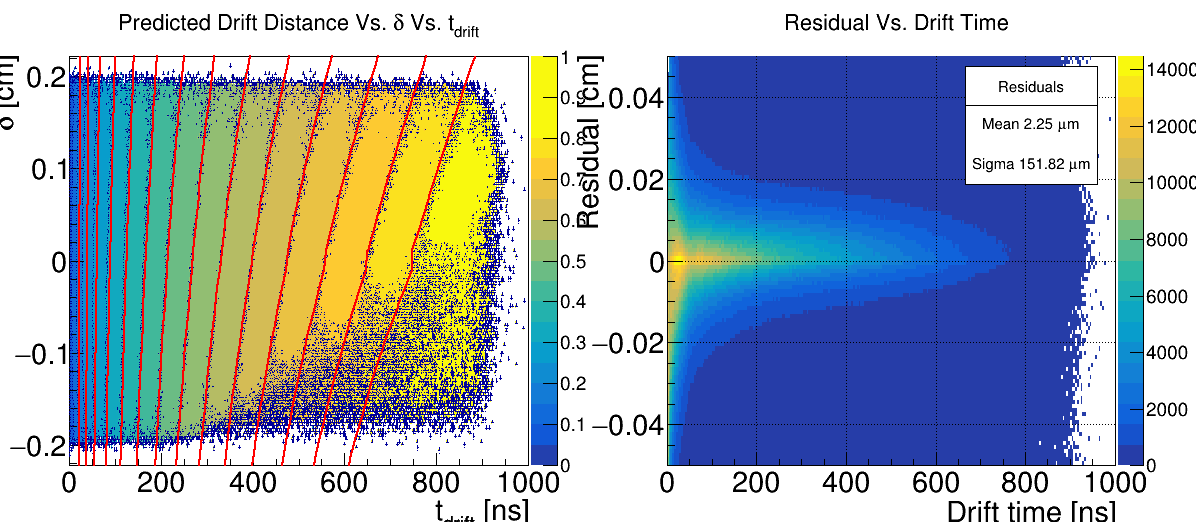
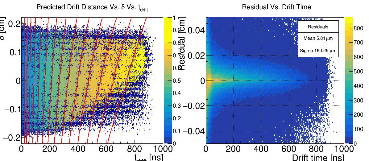
Time-to-distance: 𝛿, the change in length of the LOCA caused by the straw deformation, is
plotted against the measured drift time, t drift . The color scale indicates the distance of
closest approach between the track and the wire, obtained from the tracking software.
The red lines are contours of the time-to-distance function for constant drift distances
from 1.5 mm to 8 mm, in steps of 0.5 mm. They should lie over the top of the dark blue contour lines separating the colour blocks.
For the plot of residuals vs drift time, the mean should be less than 15um and the sigma should be less than 150um.
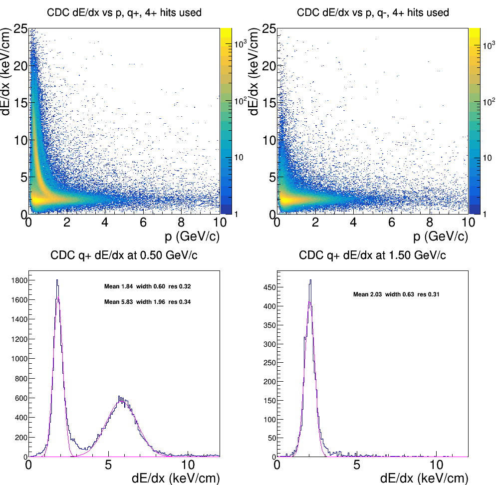
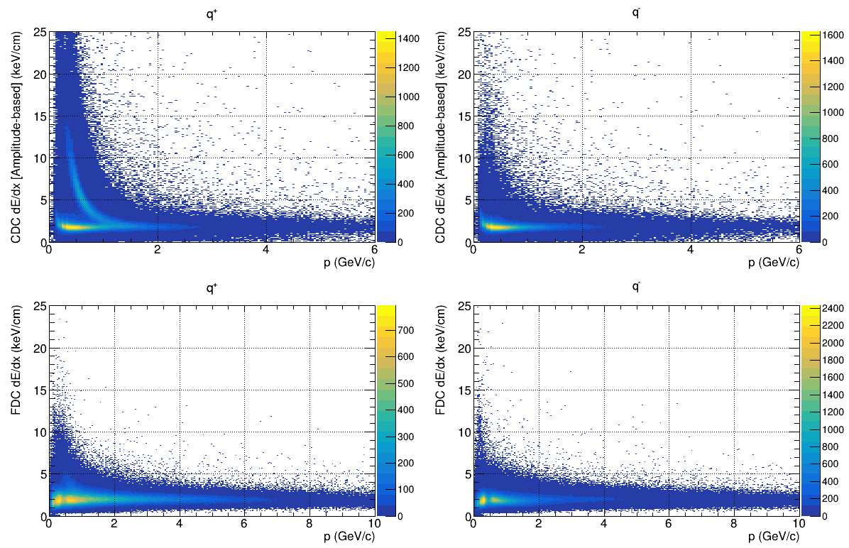
dE/dx: At 1.5GeV/c the fitted peak mean should be within 1% of 2.02 keV/cm.
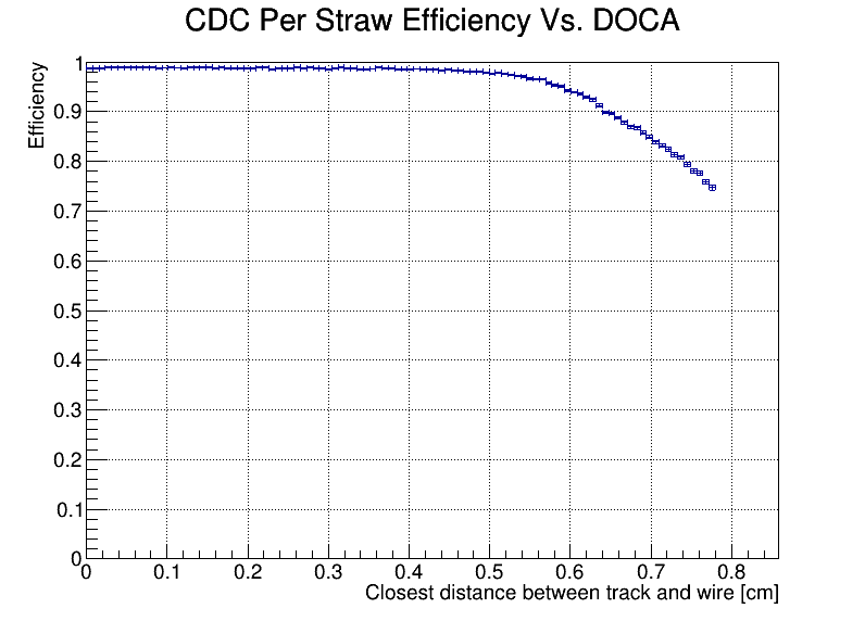
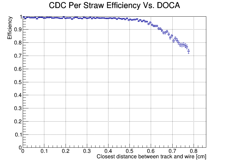
Efficiency: The efficiency should be 0.98 or higher at 0cm DOCA, gradually fall to 0.97 at approximately 0.5mm and then more steeply through 0.9 at approximately 0.64cm.
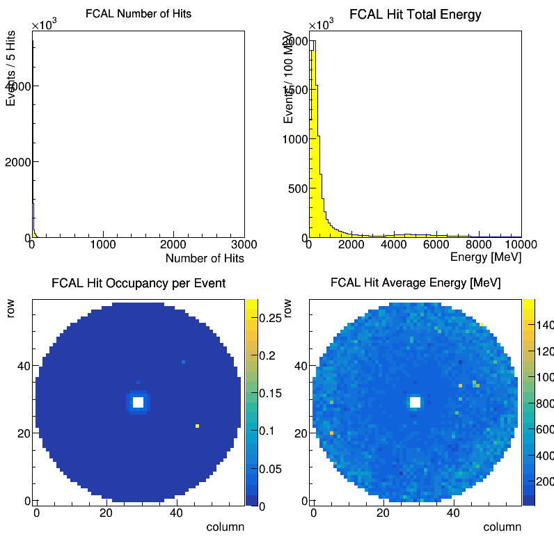
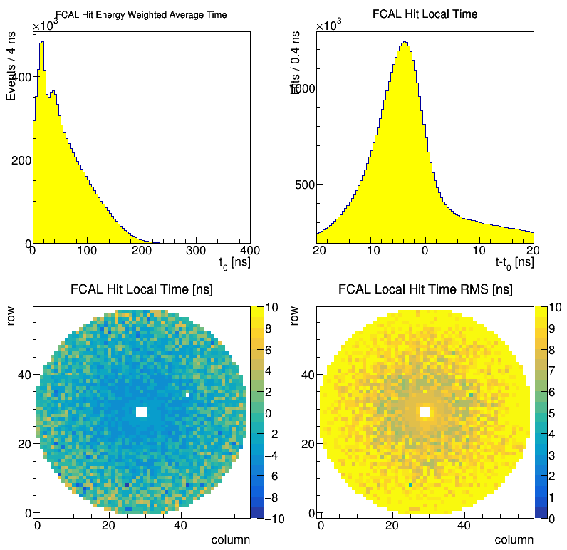
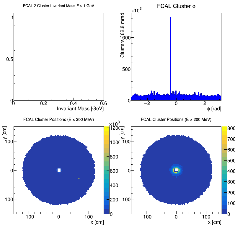
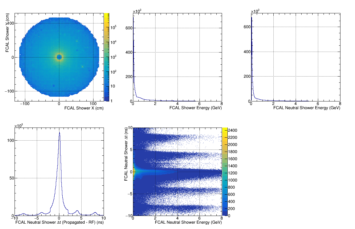
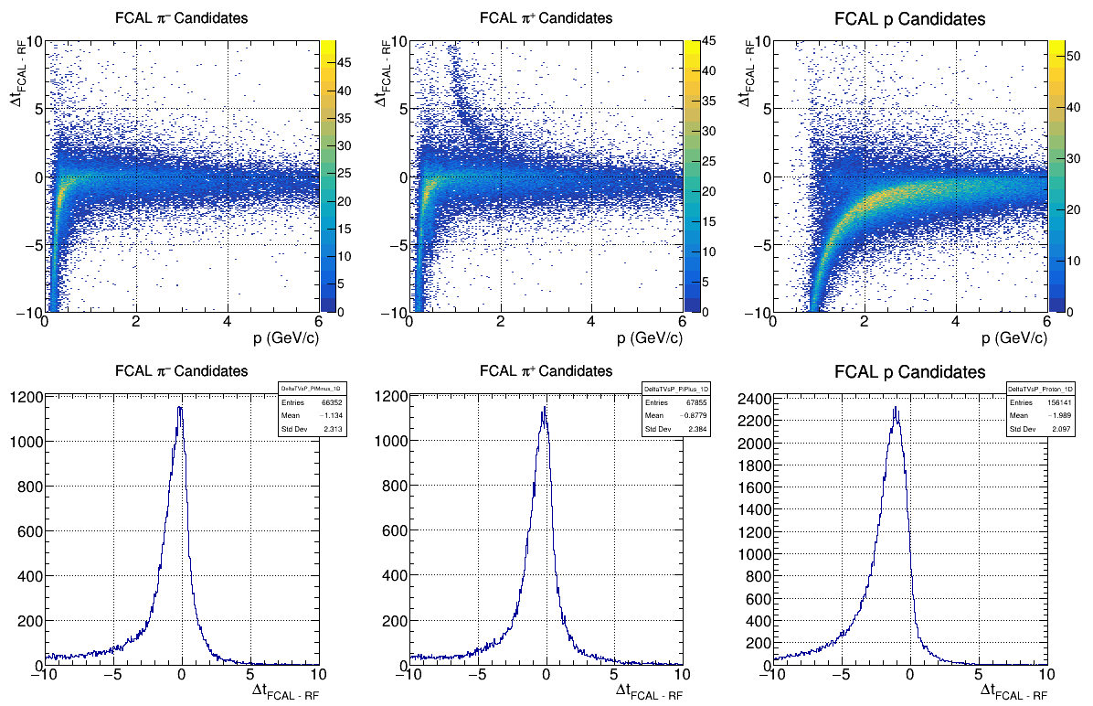
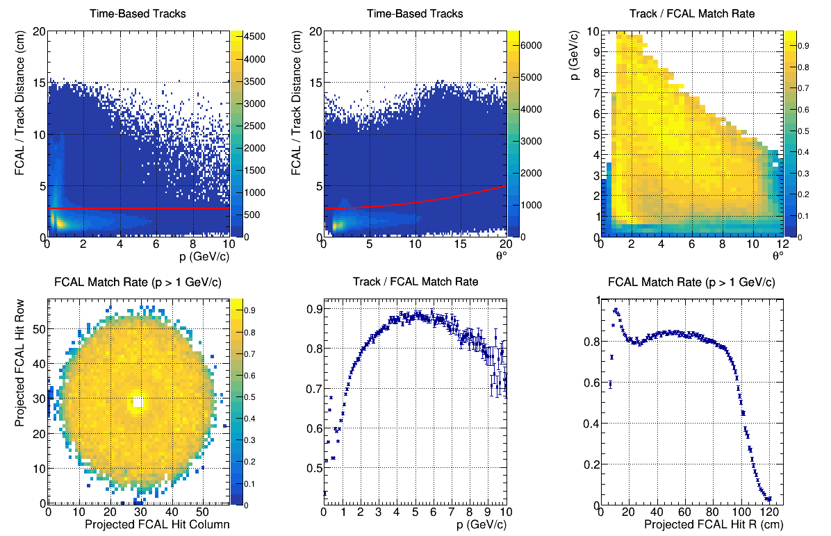
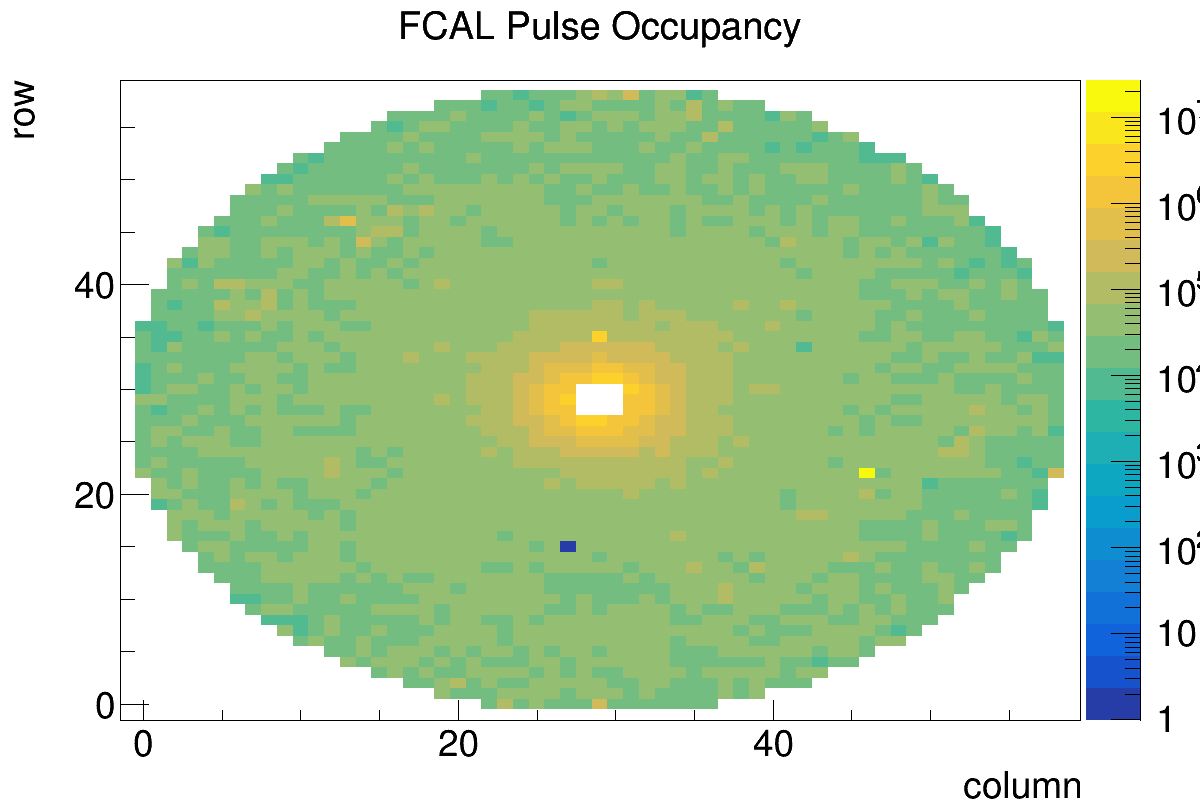
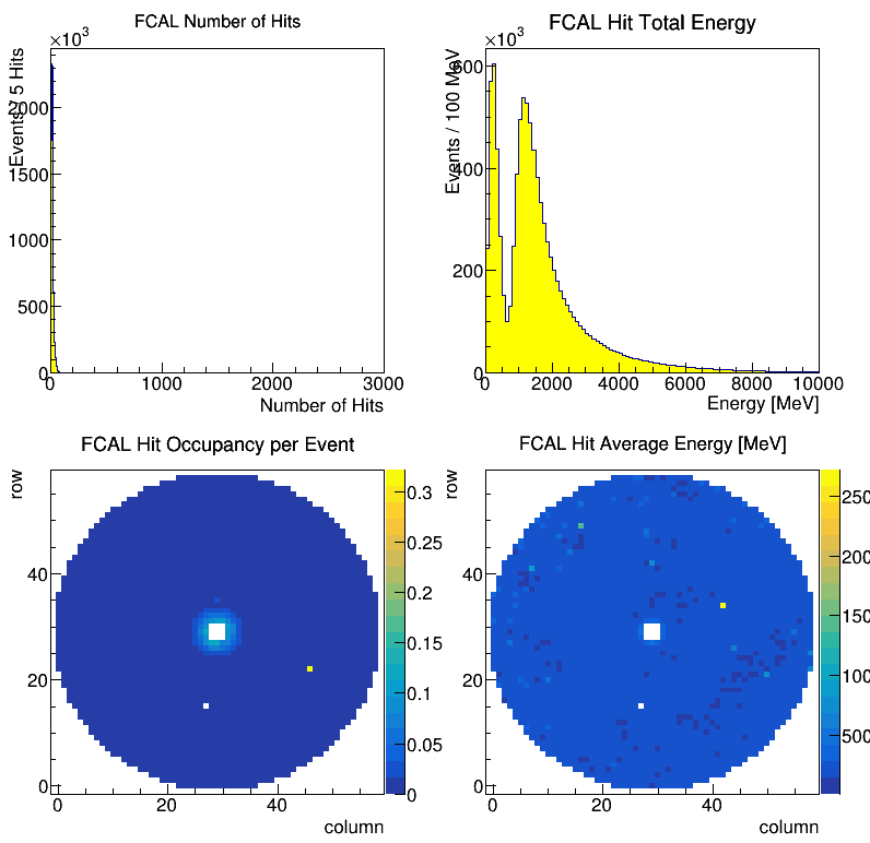
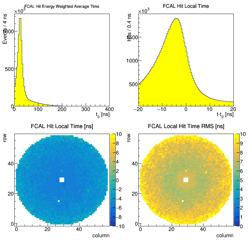
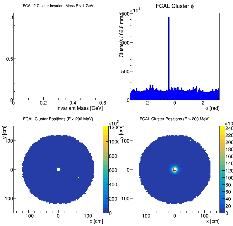
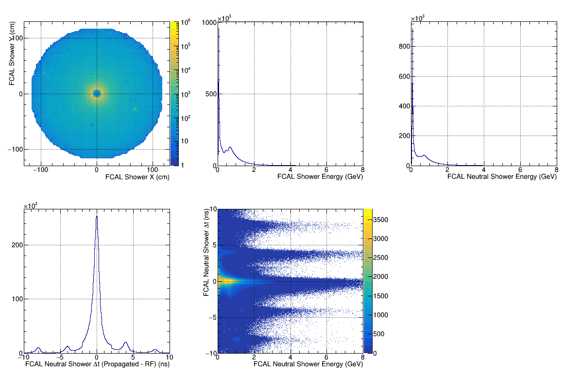
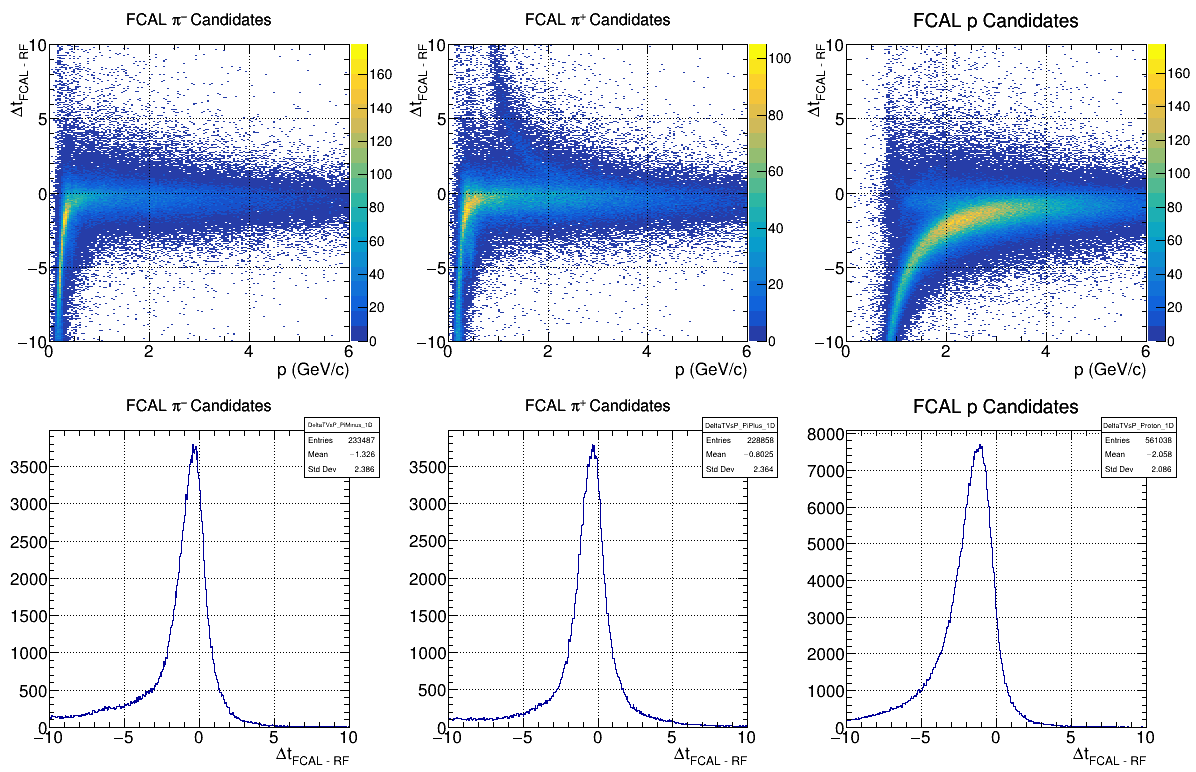
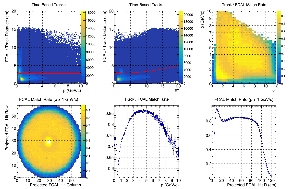
FCAL
- Check Occupancy - Reference: [ link ]
- Check FCAL Hits 1 - Reference: [ link ]
- Check FCAL Hits 2 - Reference: [ link ]
- Check FCAL Clusters 1 - Reference: [ link ]
- Check FCAL Recon. 1 - Reference: [ link ]
- Check FCAL Recon. 2 - Reference: [ link ]
- Check Recon. FCAL Matching - Reference: [ link ]
FCAL Reference Plots
Beryllium Target


Full Liquid Helium Target
Empty Liquid Helium Target
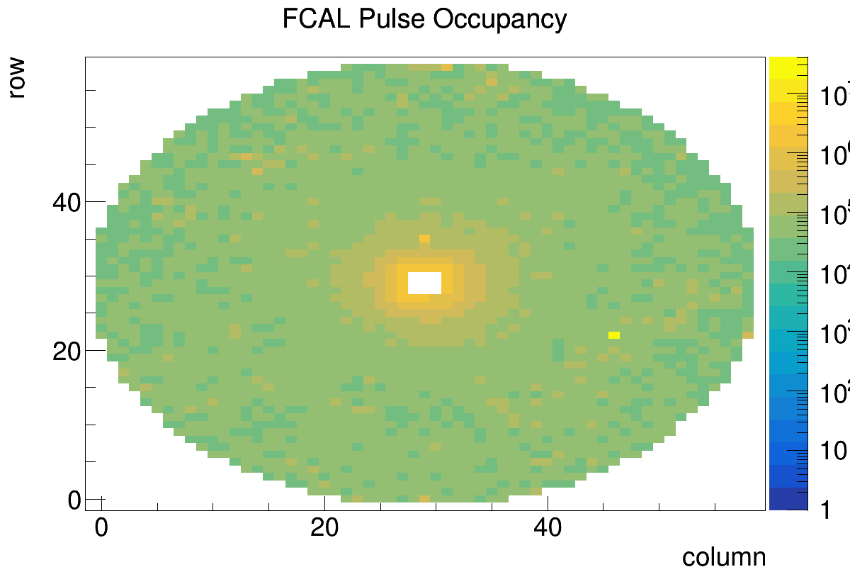
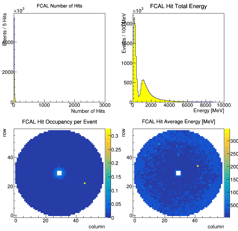
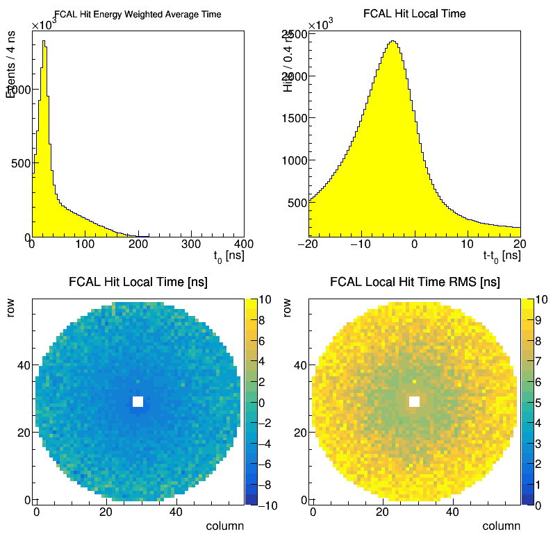
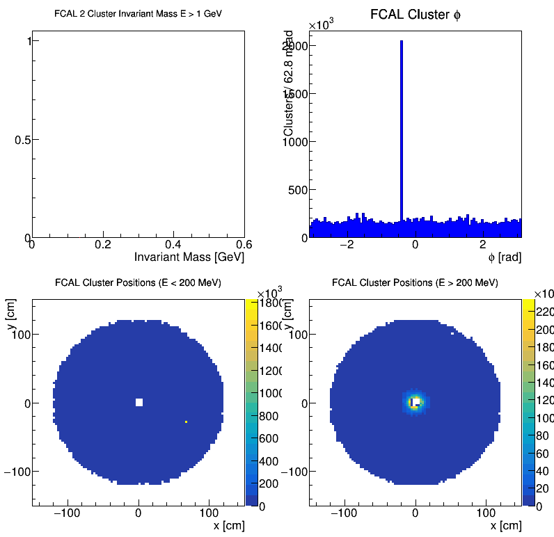
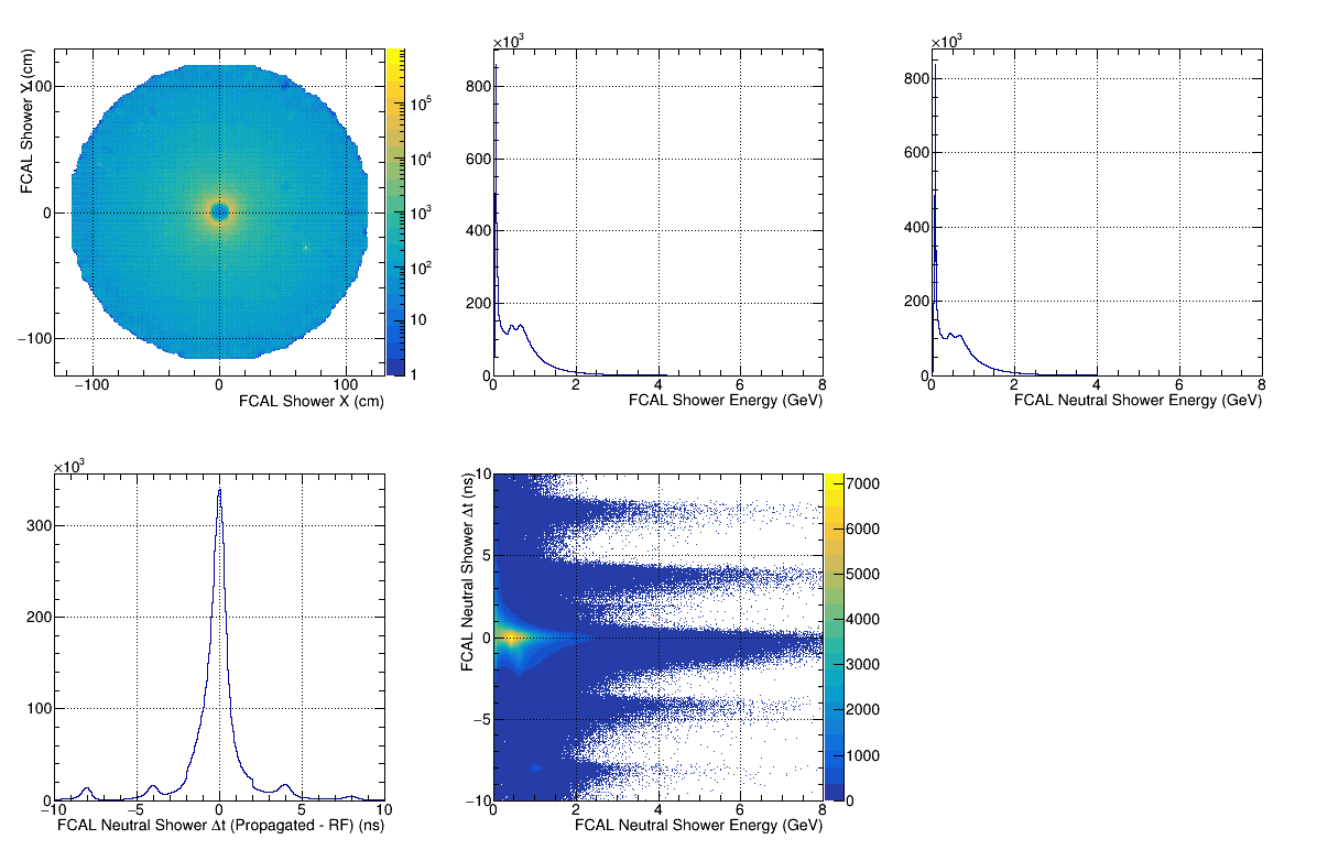
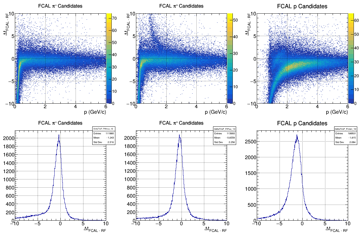
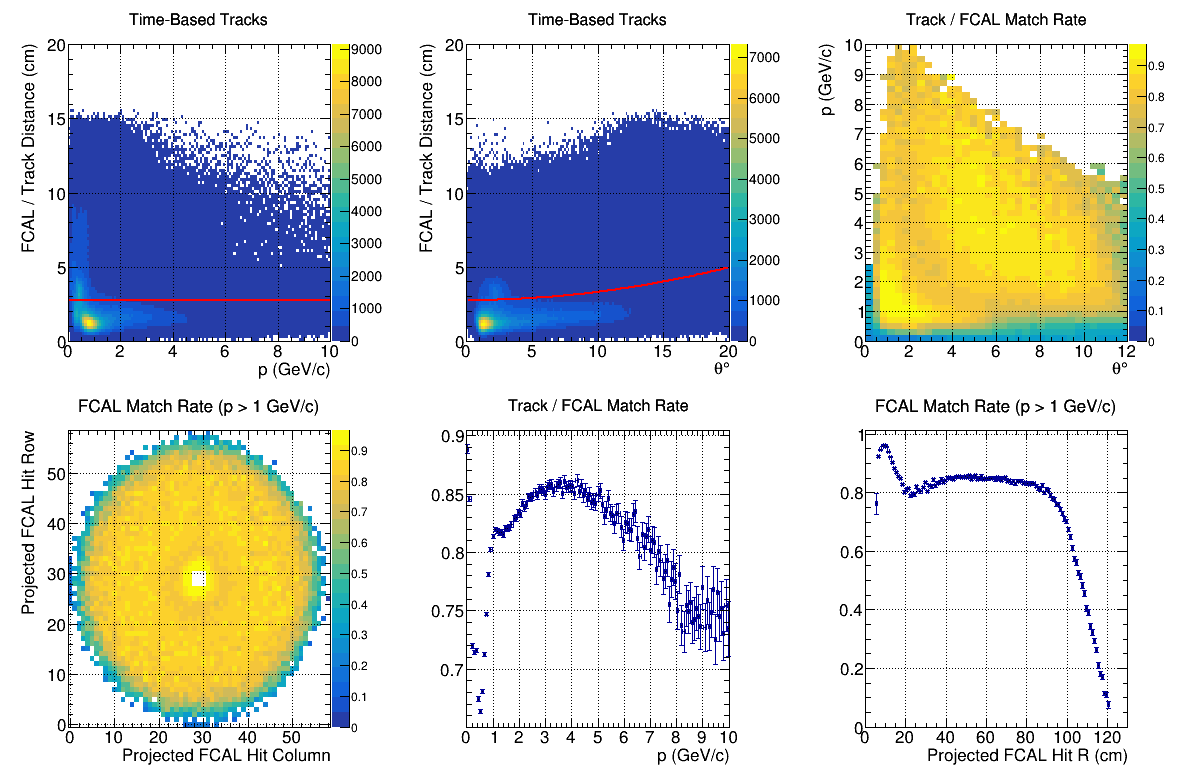
FCAL Notes
Instructions for monitoring volunteers go here.
FDC
- Check Package 1 Occupancy - Reference: [ link ]
- Check Package 2 Occupancy - Reference: [ link ]
- Check Package 3 Occupancy - Reference: [ link ]
- Check Package 4 Occupancy - Reference: [ link ]
FDC Reference Plots
Beryllium Target


Full Liquid Helium Target
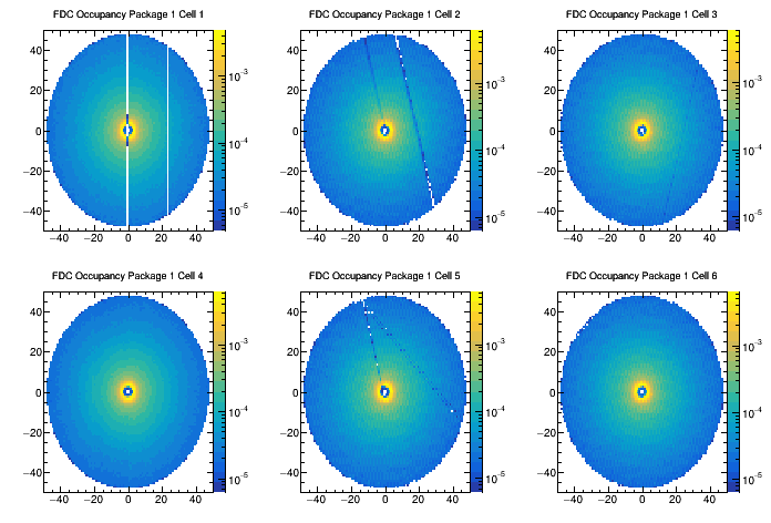

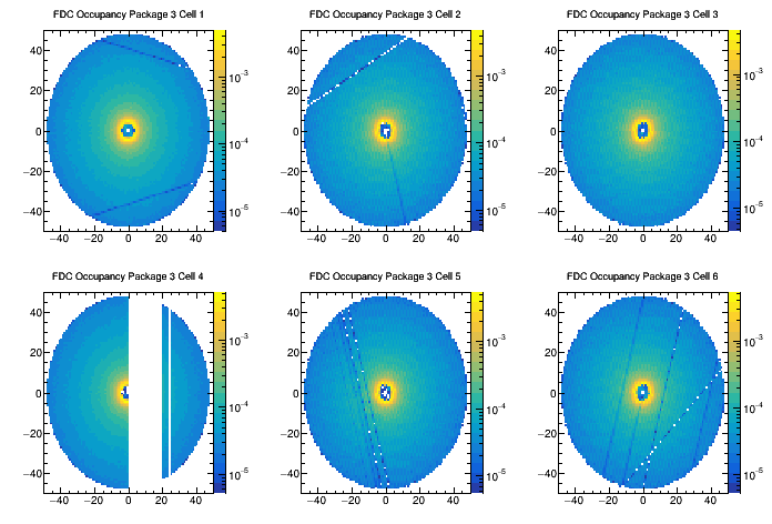
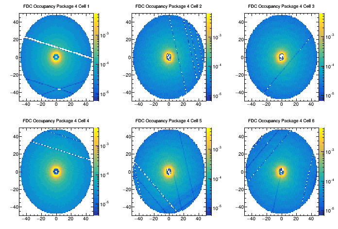
Empty Liquid Helium Target
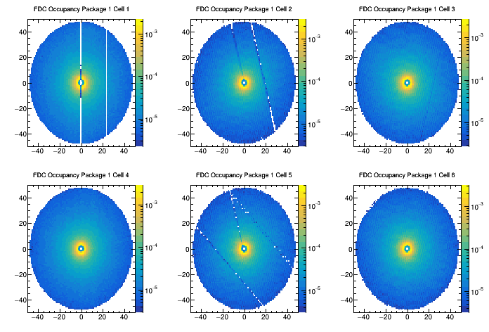
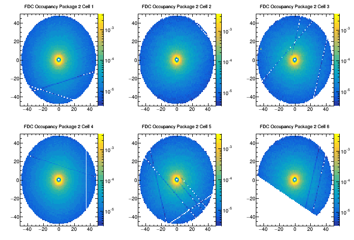
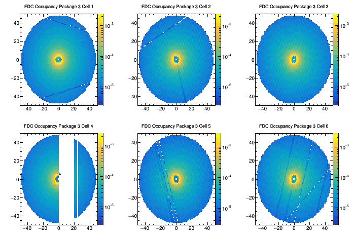
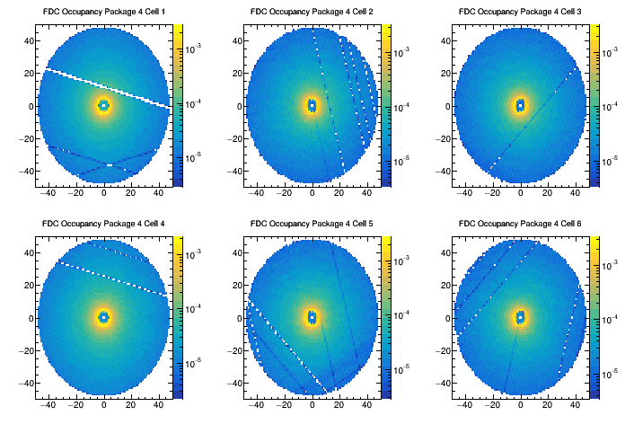
FDC Notes
Instructions for monitoring volunteers go here.
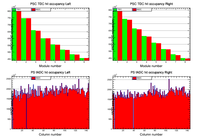
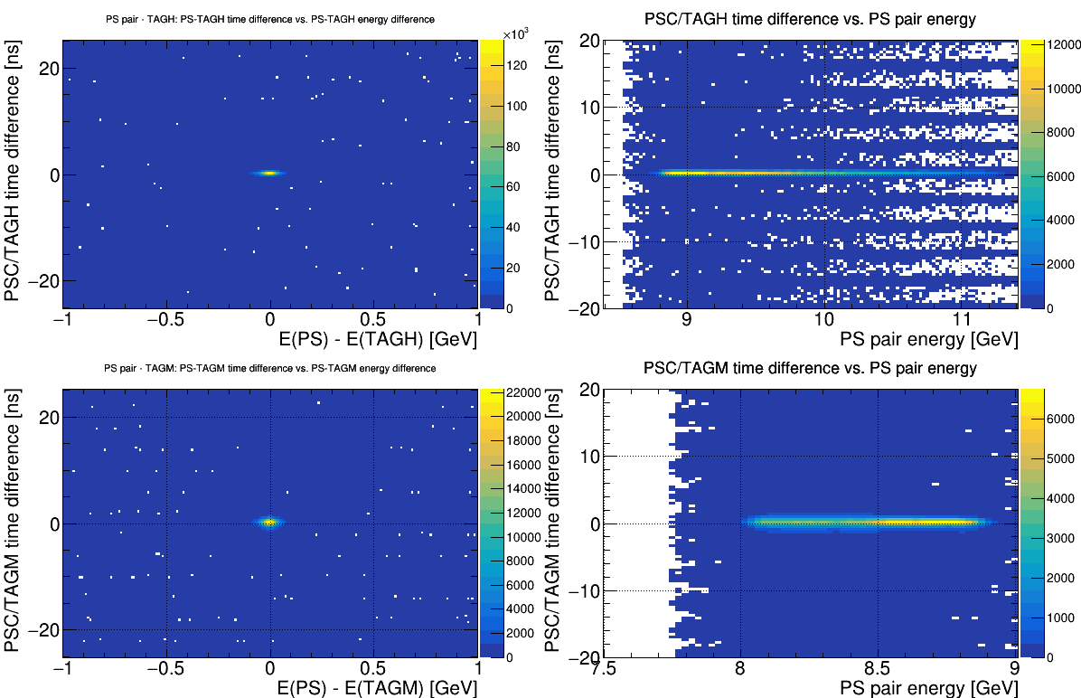
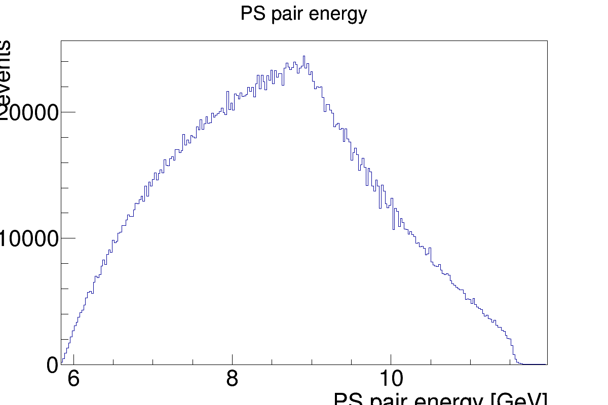
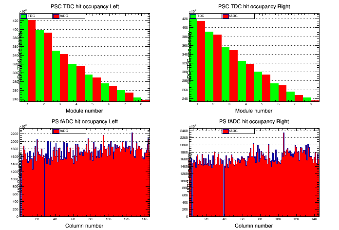
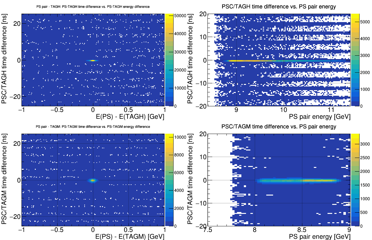
PS
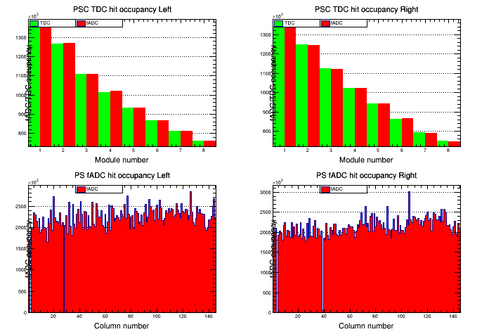
- Check Occupancy - Reference: [ link ]
- Check Timing Alignment - Reference: [ link ]
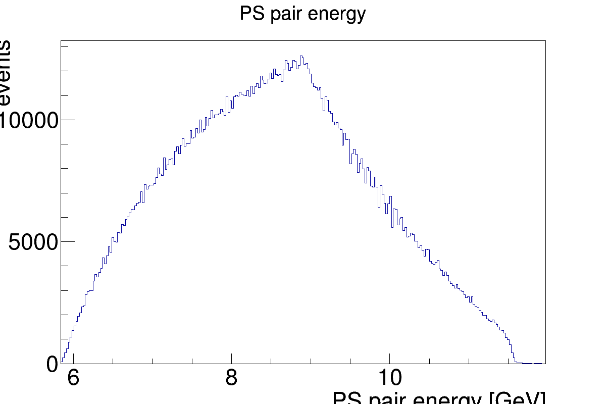
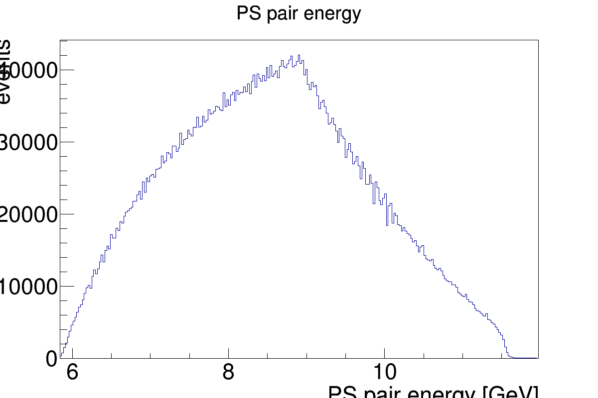
- Check PS Pair Energy - Reference: [ link ]
PS Reference Plots
Beryllium Target


Full Liquid Helium Target
Empty Liquid Helium Target

PS Notes
PS Occupancy: PS Occupancy (bottom) should be fairly flat with a couple bad channels. PSC Occupancy (top) should have similar rates in TDC and ADC, with the same shape as the reference histogram. PS Timing: All plots should be centered at zero. The right column reflect the tagger energy, the bottom right is empty (should be updated?). PS Pair Energy: Should have similar triangle-like shape as the reference.
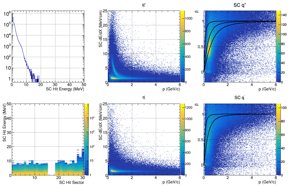
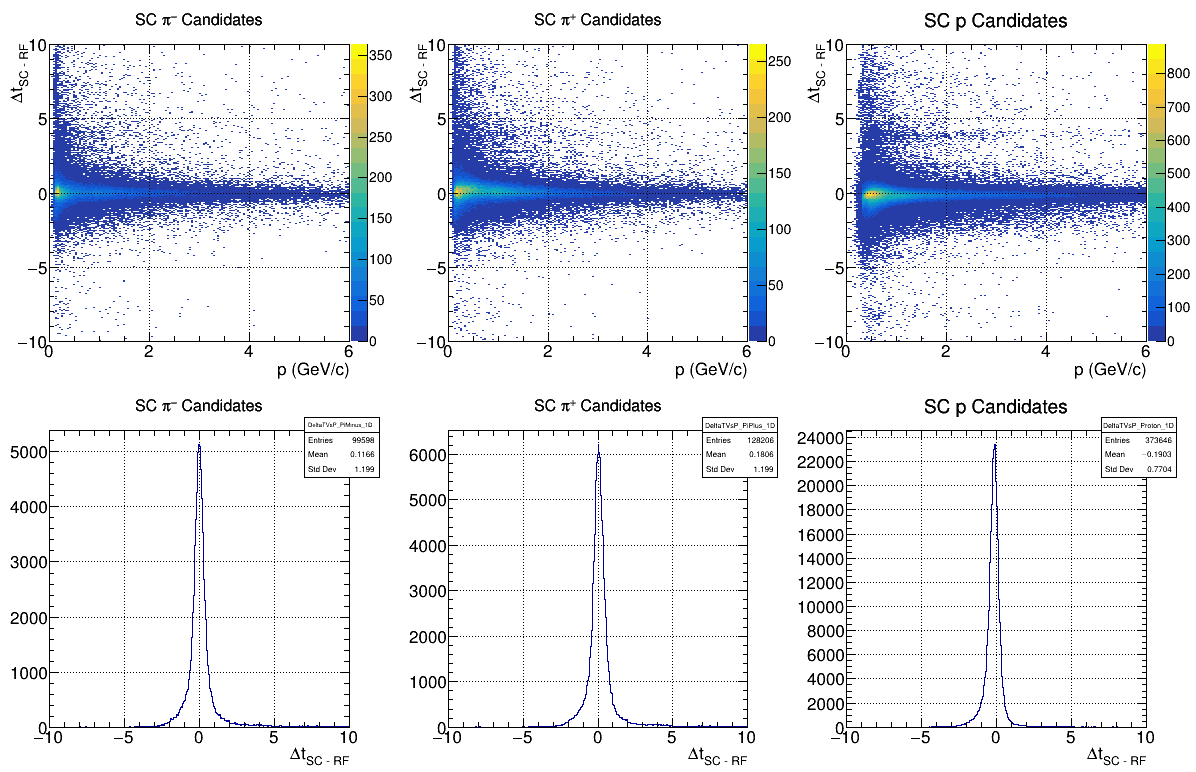
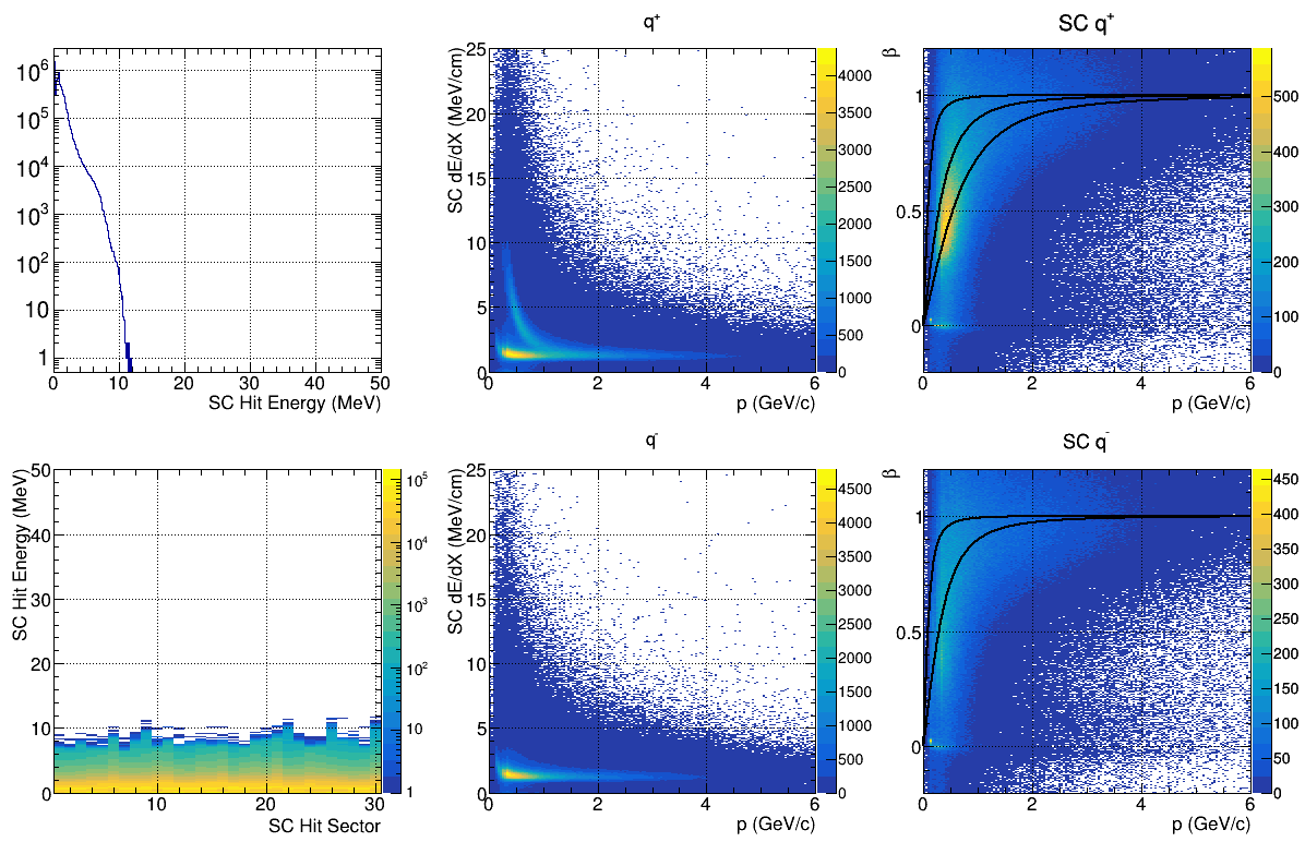
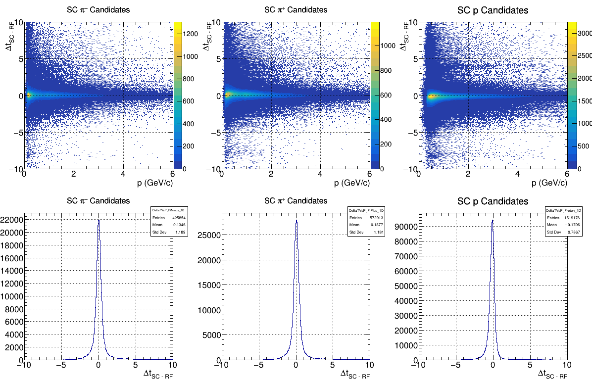
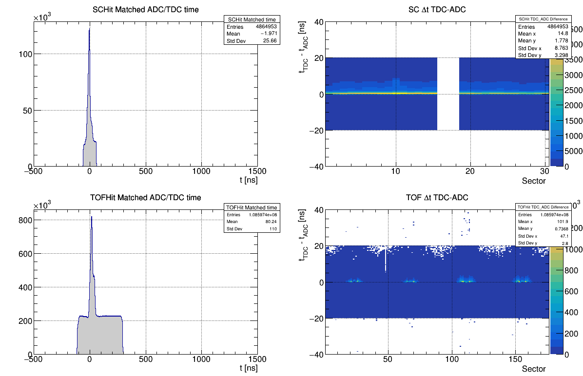
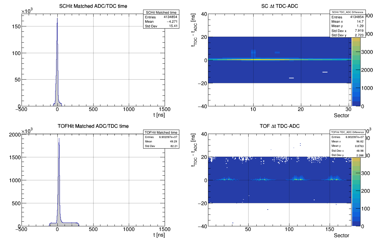
SC
- Check Occupancy - Reference: [ link ]
- Check Recon. SC 1 - Reference: [ link ]
- Check Recon. SC 2 - Reference: [ link ]
- Check Recon. SC Matching - Reference: [ link ]
SC Reference Plots
Beryllium Target


Full Liquid Helium Target
Empty Liquid Helium Target
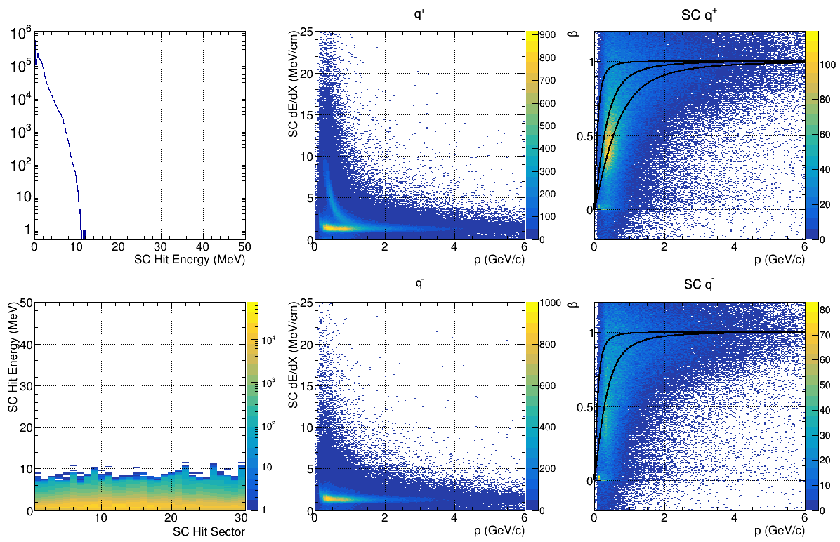
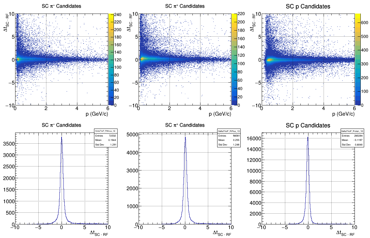
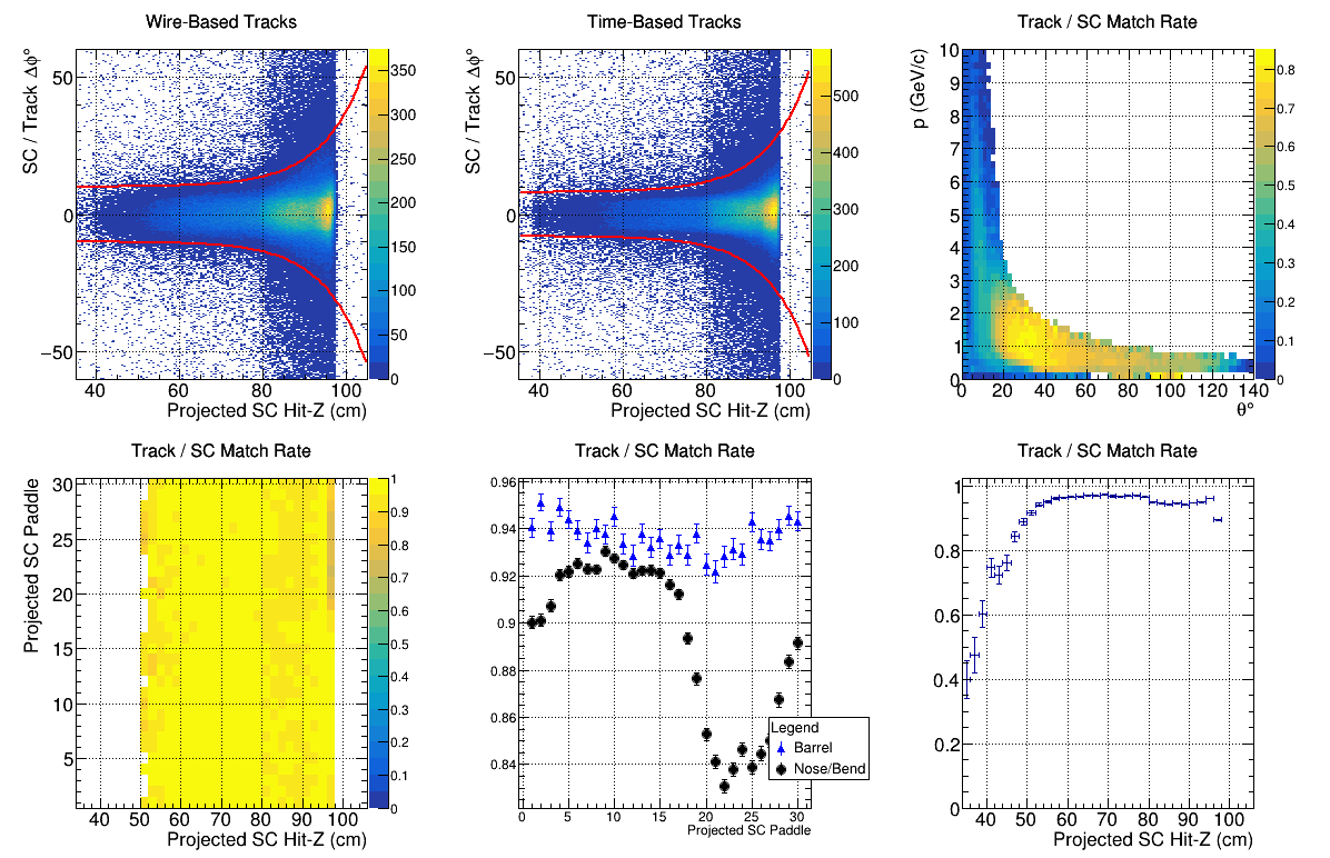
SC Notes
Instructions for monitoring volunteers go here
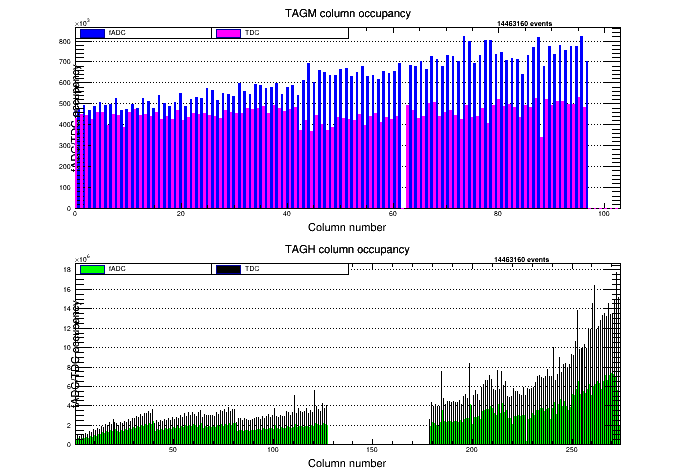
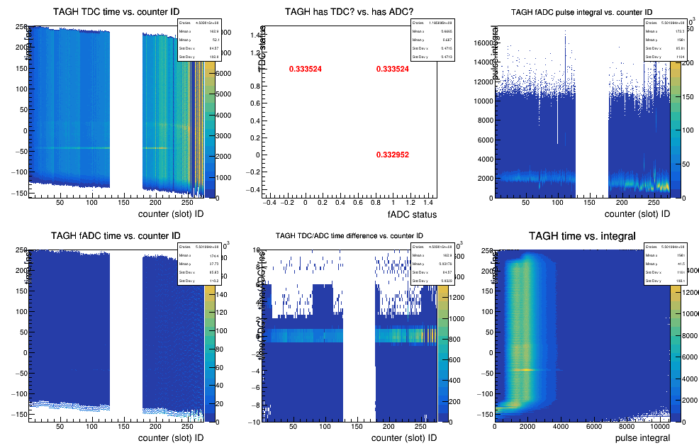
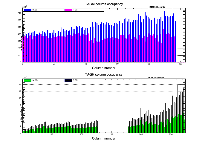
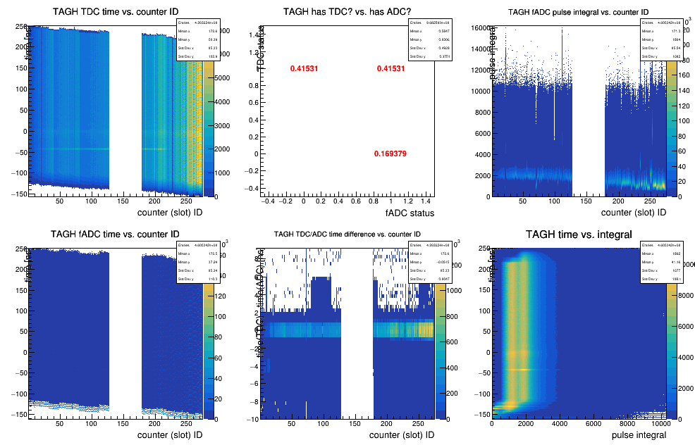
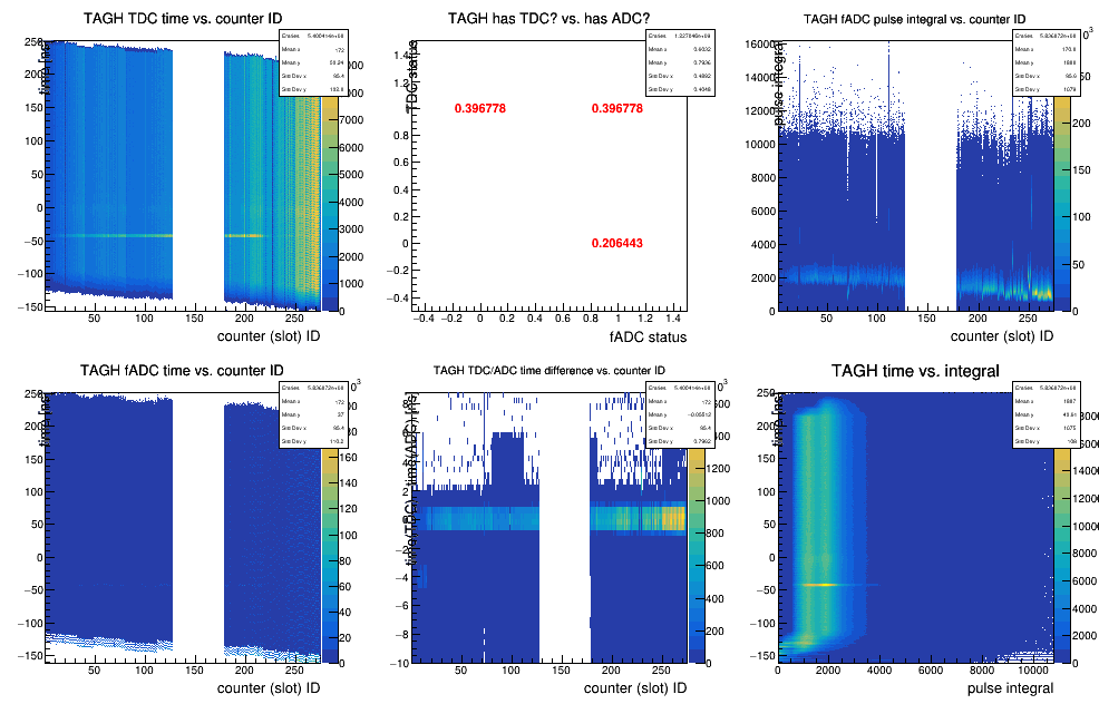
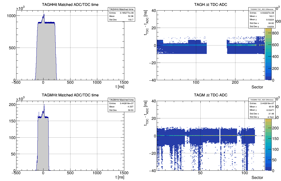
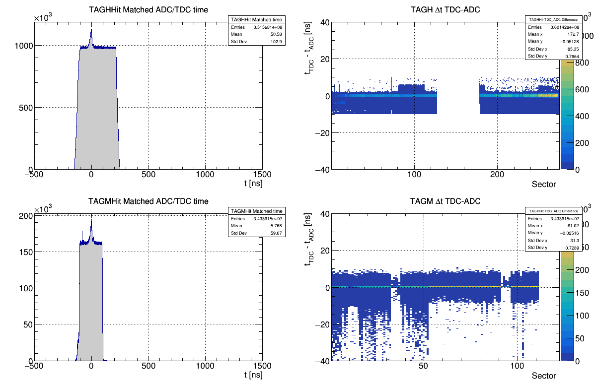
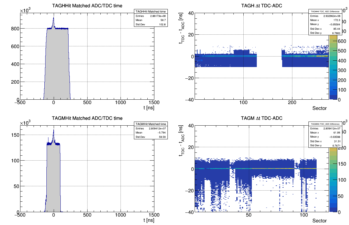
TAGH
TAGH Reference Plots
Beryllium Target


Full Liquid Helium Target
Empty Liquid Helium Target

TAGH Notes
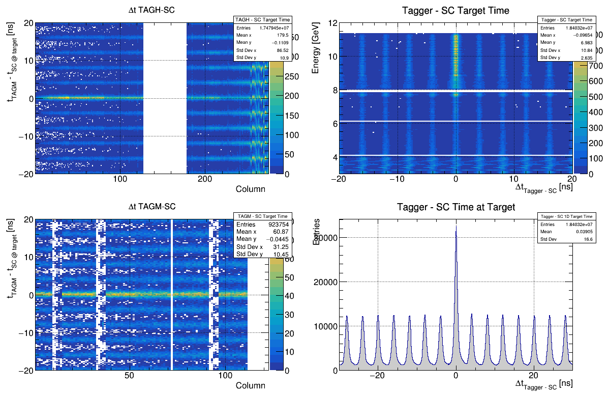
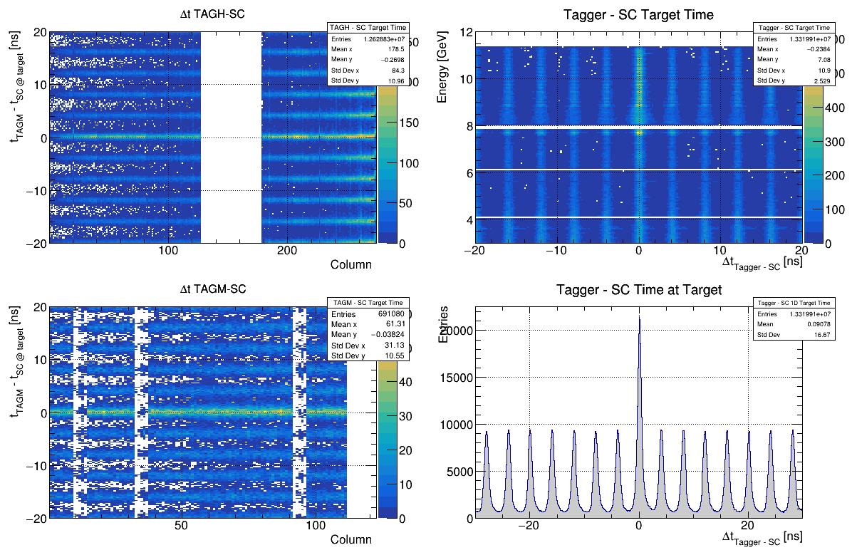
Tagger occupancy: TAGM - Generally the fADC and TDC occupancies should be similar and mostly flat, with maybe a small increase in rates with column number. There can be a small step in the TDC occupancy. TAGH - expect the choppy pattern in the reference image, which reflects the varying size of the different counters, and a steep increase at large counter number. TAGH Hits 2: This plot is complicated - the main thing to look for is the time(TDC)-time(ADC) vs. channel plot to be centered around zero. Keep an eye out for any extra or unusual dead channels.
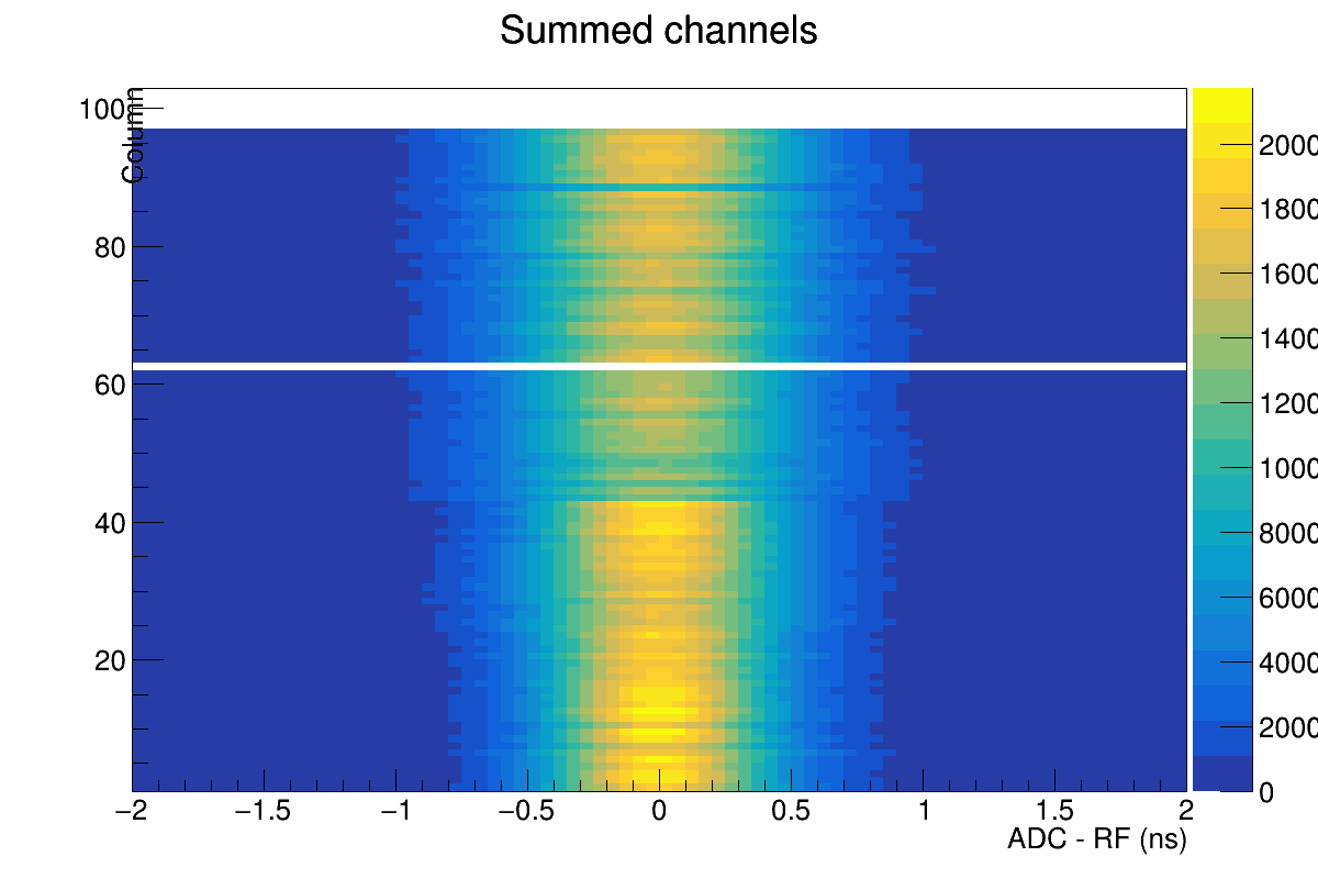
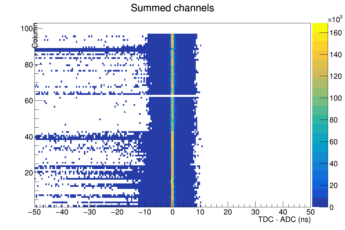
TAGM
TAGM Reference Plots
Beryllium Target


Full Liquid Helium Target
Empty Liquid Helium Target
TAGM Notes
Generally both distributions should be centered near zero. There is some variation in intensity due to the shape of the photon beam energy dependence (coherent peak) and the inefficiency of some of the channels.
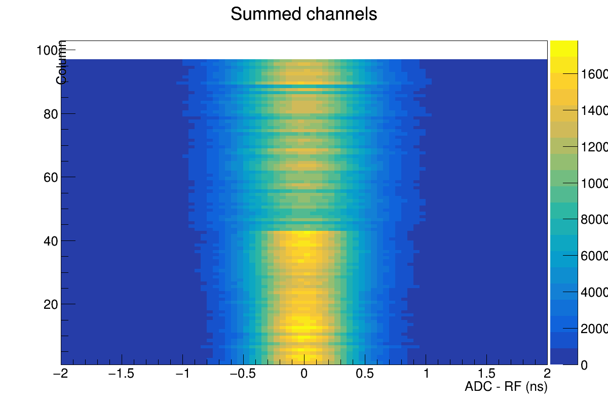
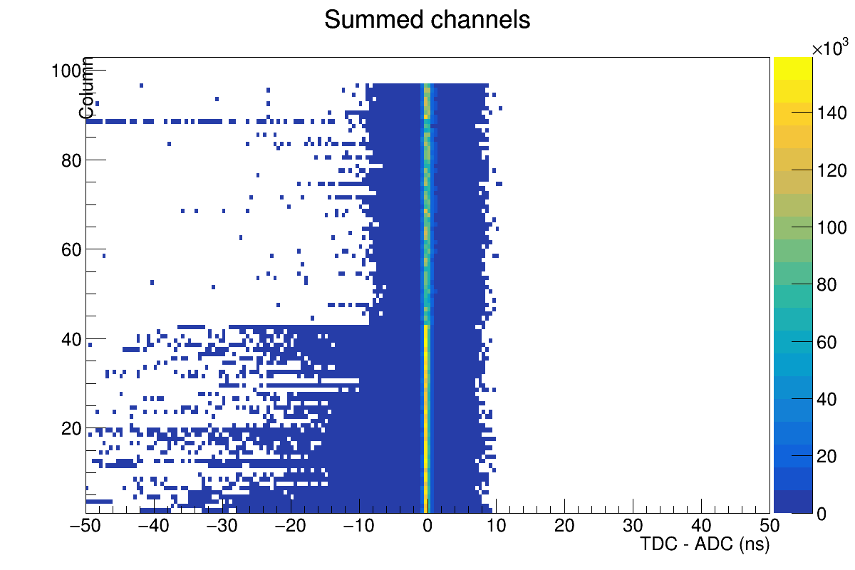
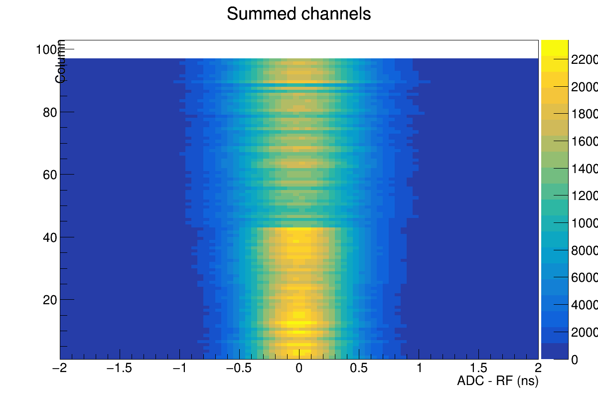
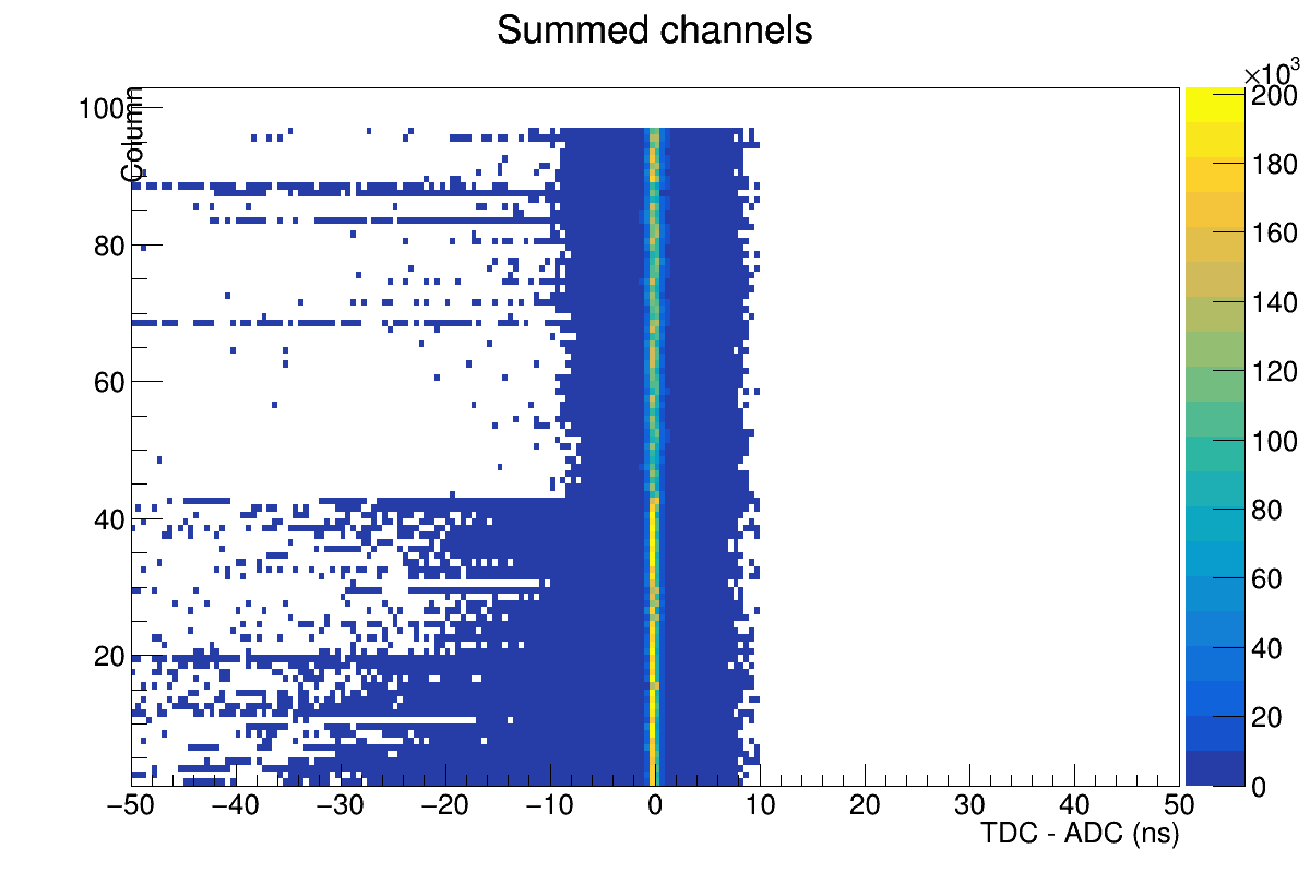
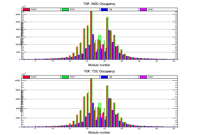
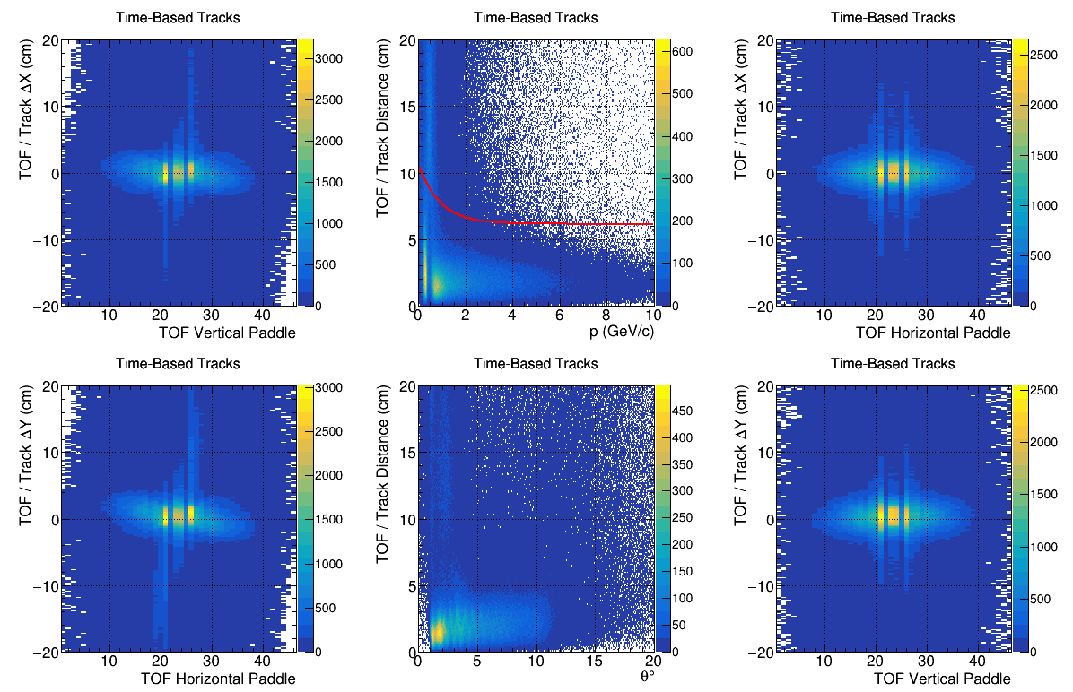
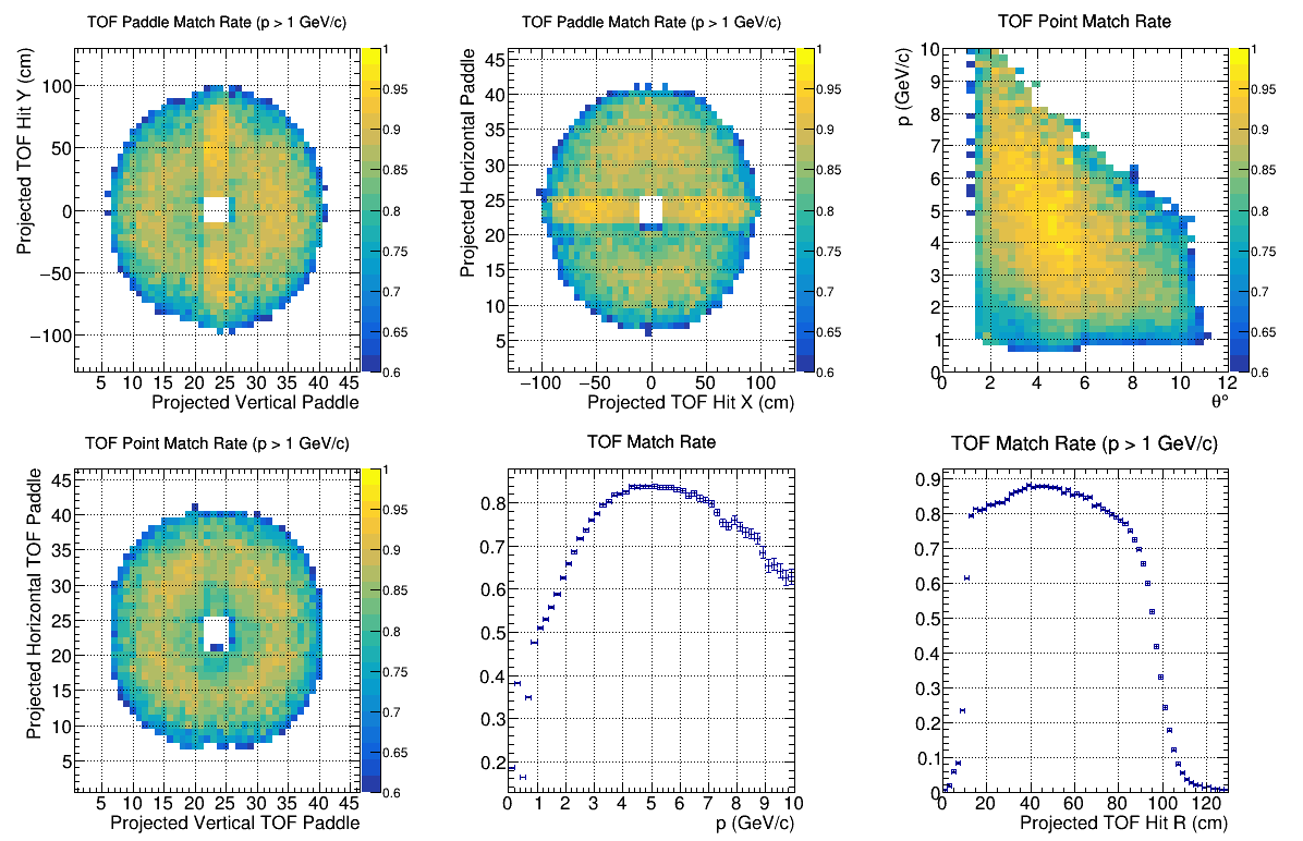
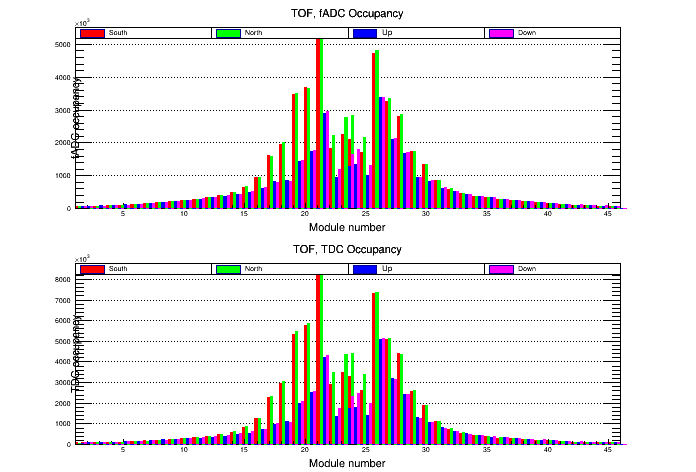
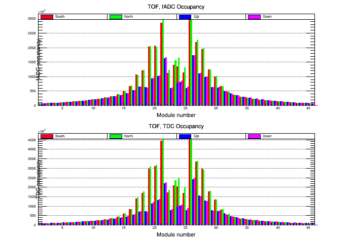
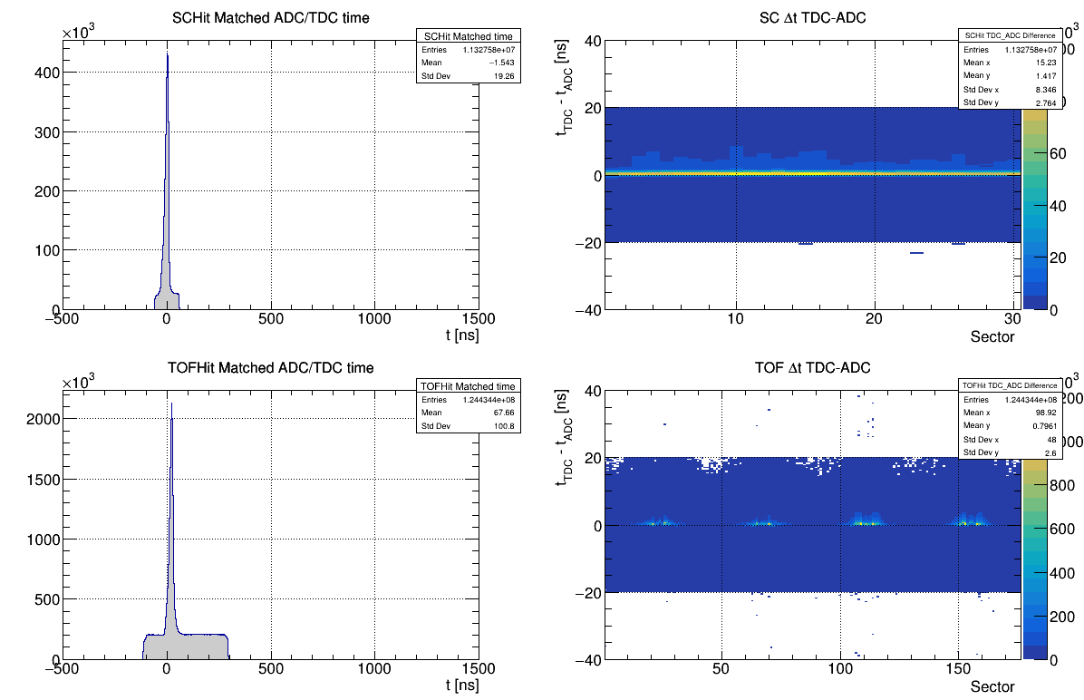
TOF
- Check Occupancy - Reference: [ link ]
- Check TOF Matching 1 - Reference: [ link ]
- Check TOF Matching 2 - Reference: [ link ]
TOF Reference Plots
Beryllium Target


Full Liquid Helium Target
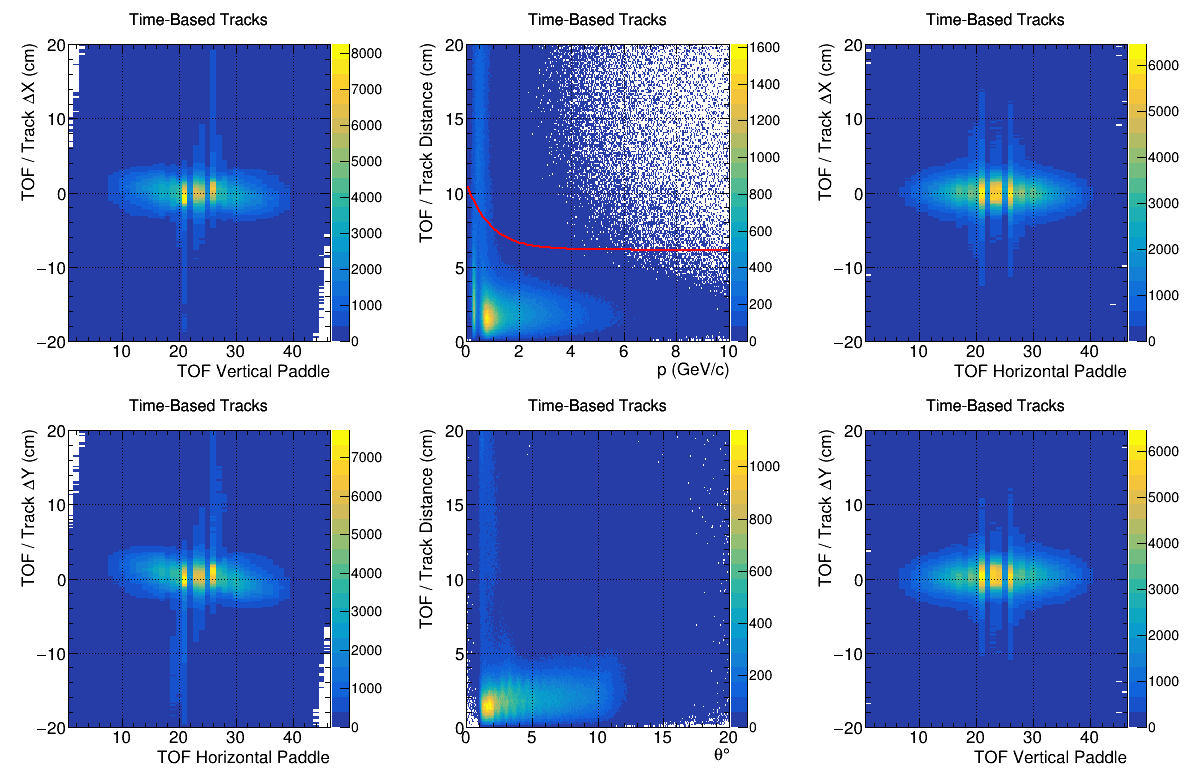
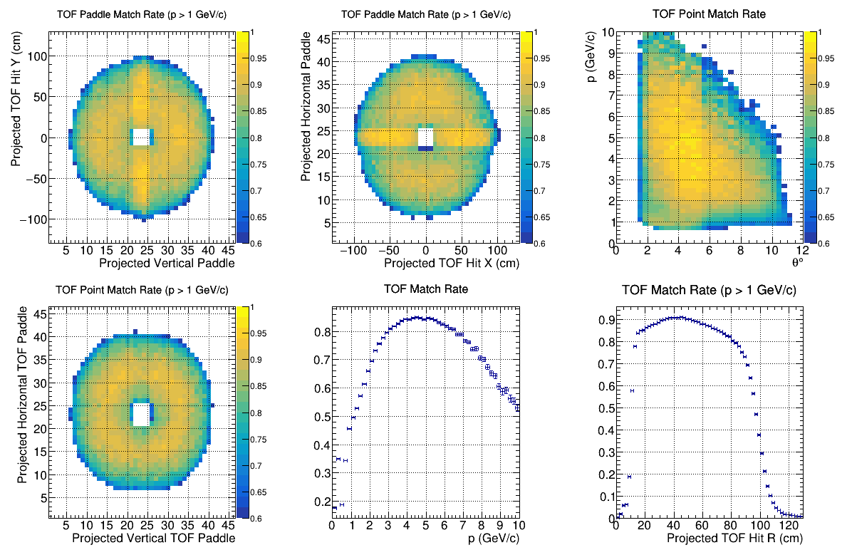
Empty Liquid Helium Target
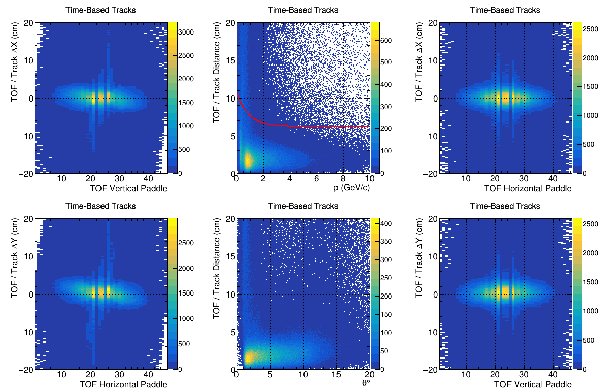
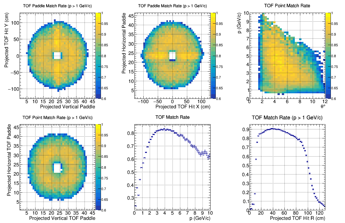
TOF Notes
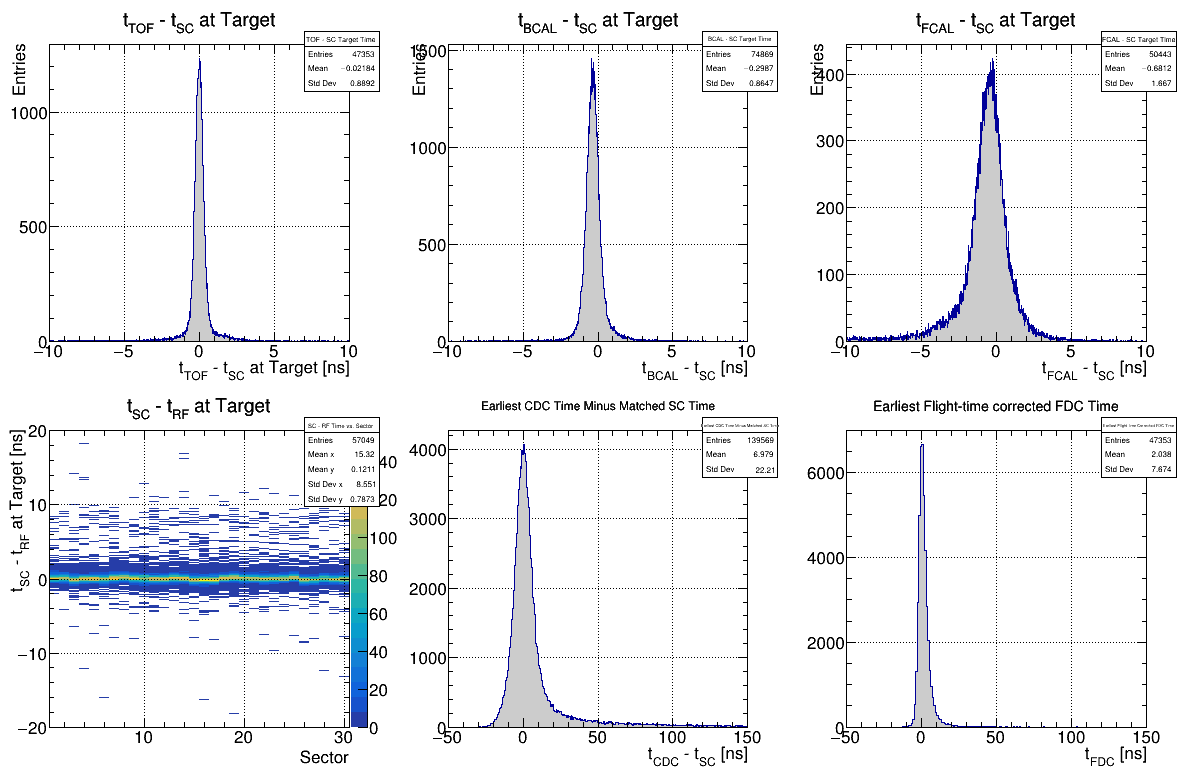
*Occupancy plot: look for "gaps" indicative of missing counters *Matching TOF Hits: X and Y (right most plots) distributions should be centered close to zero (vertical) *TOF mathching in 1d histograms should have regions larger than 80%
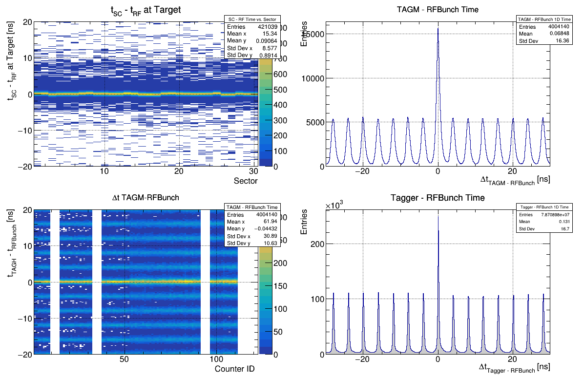
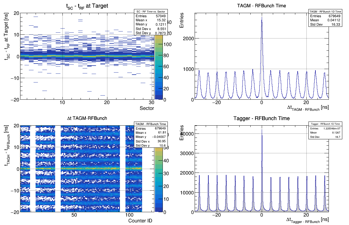
RF
- Check Timing Offsets - Reference: [ link ]
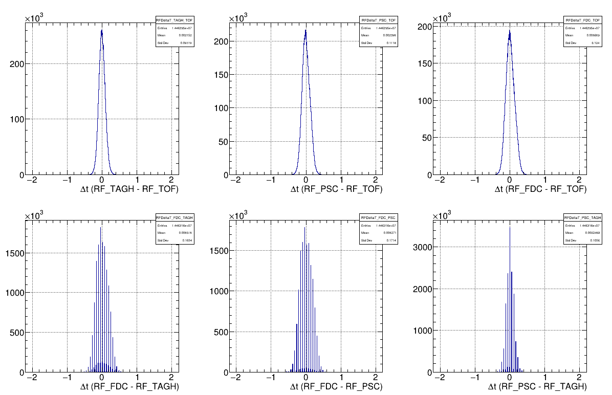
RF Reference Plots
Beryllium Target

Full Liquid Helium Target
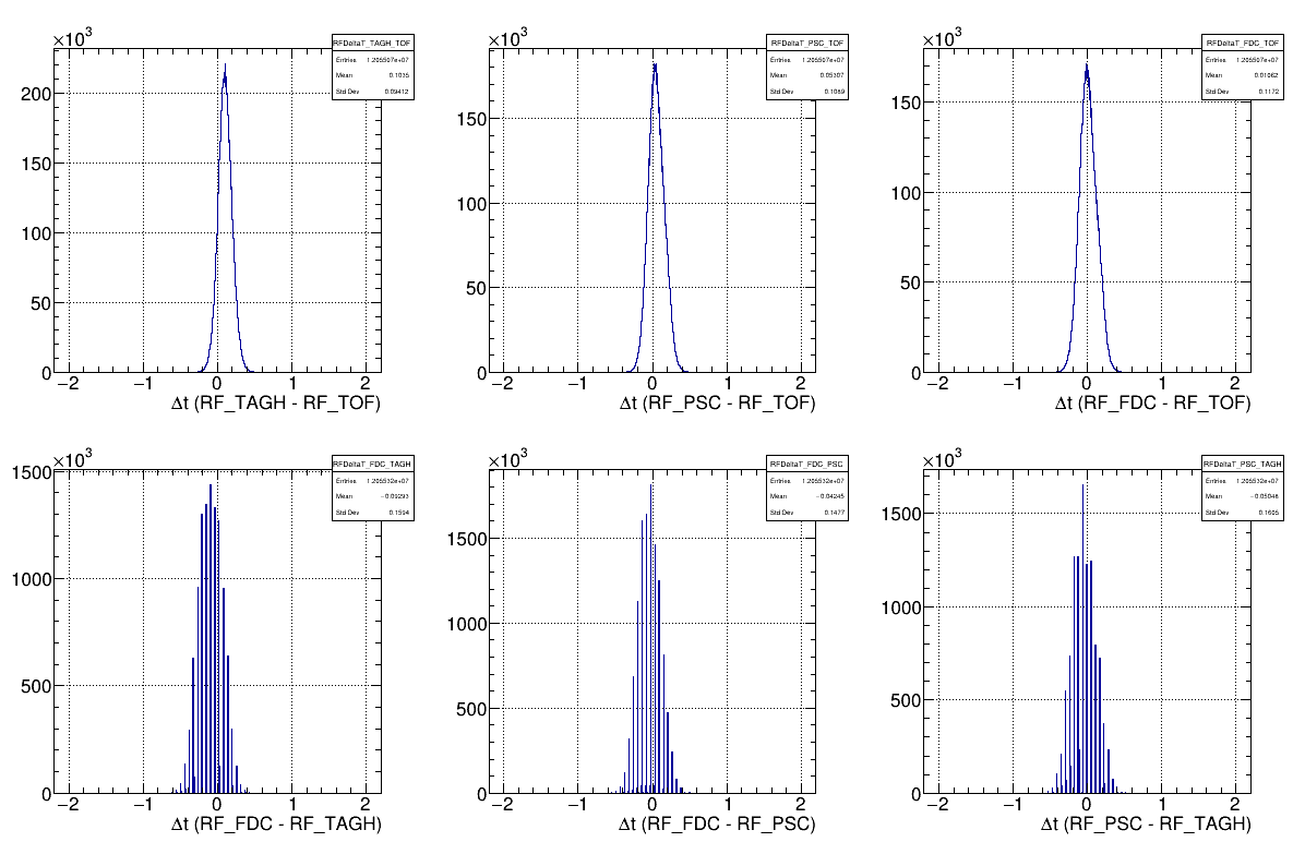
Empty Liquid Helium Target
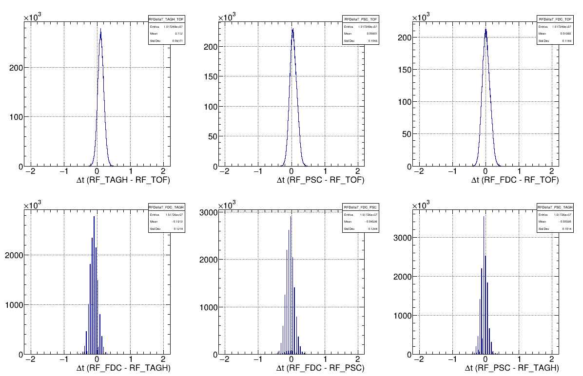
RF Instructions
Should be centered around zero.
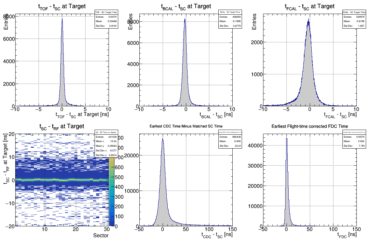
Timing
- Check HLDT Calorimeter Timing - Reference: [ link ]
- Check HLDT Drift Chamber Timing - Reference: [ link ]
- Check HLDT PID System Timing - Reference: [ link ]
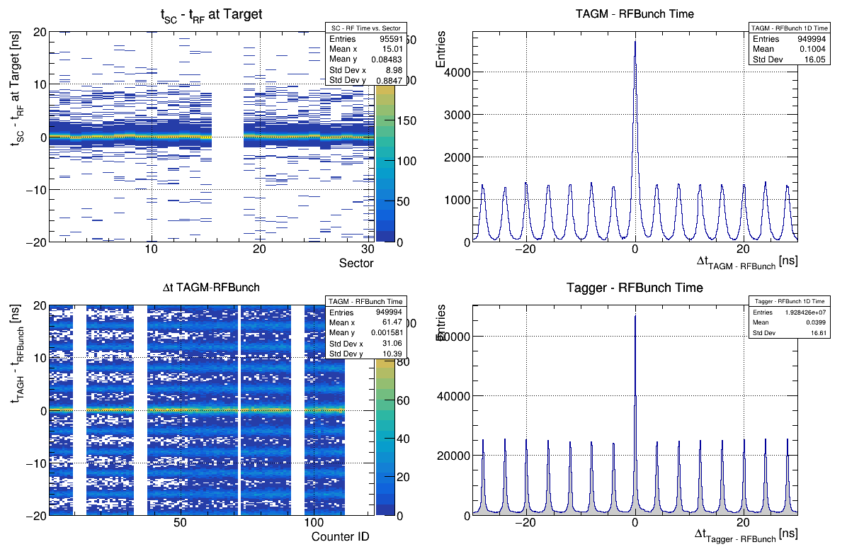
- Check HLDT Tagger Timing - Reference: [ link ]
- Check HLDT Tagger/RF Align 2 - Reference: [ link ]
- Check HLDT Tagger/SC Align - Reference: [ link ]
- Check HLDT Track-Matched Timing - Reference: [ link ]
Timing Reference Plots
Beryllium Target

![]()


Full Liquid Helium Target
![]()

Empty Liquid Helium Target
![]()
Timing Notes
Note that the relative size of peaks can change between different running conditions.
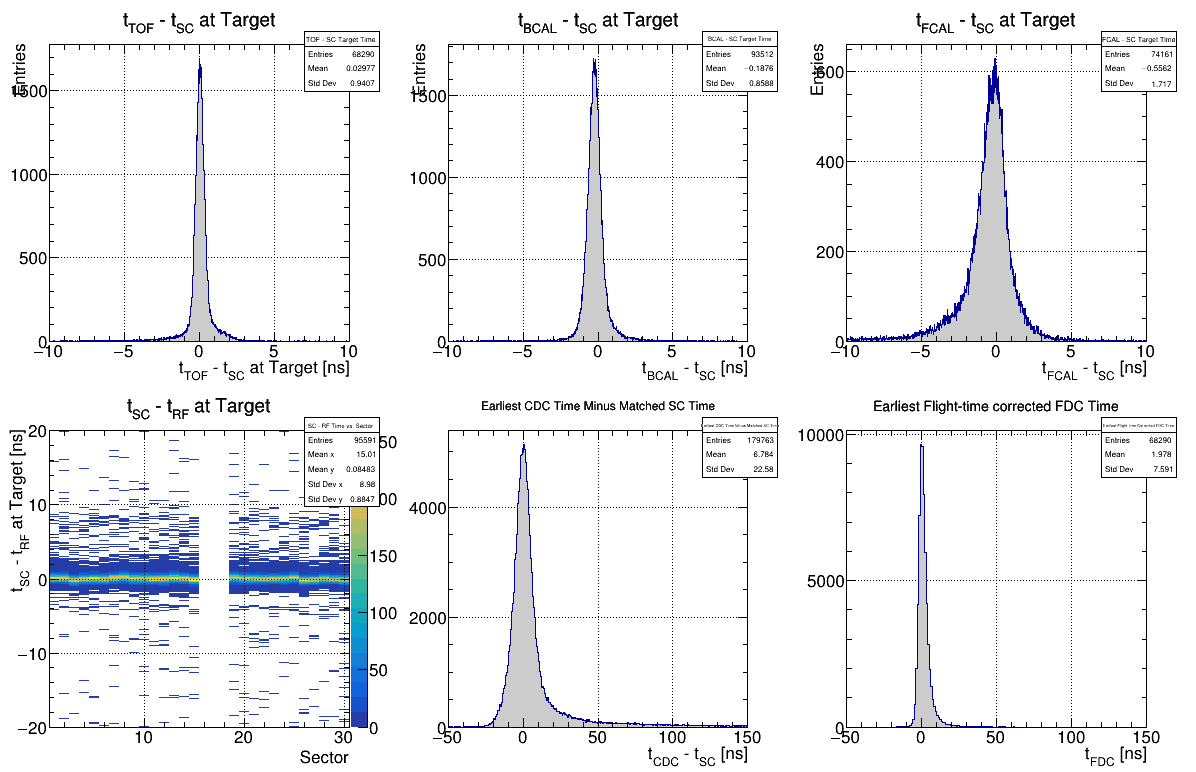
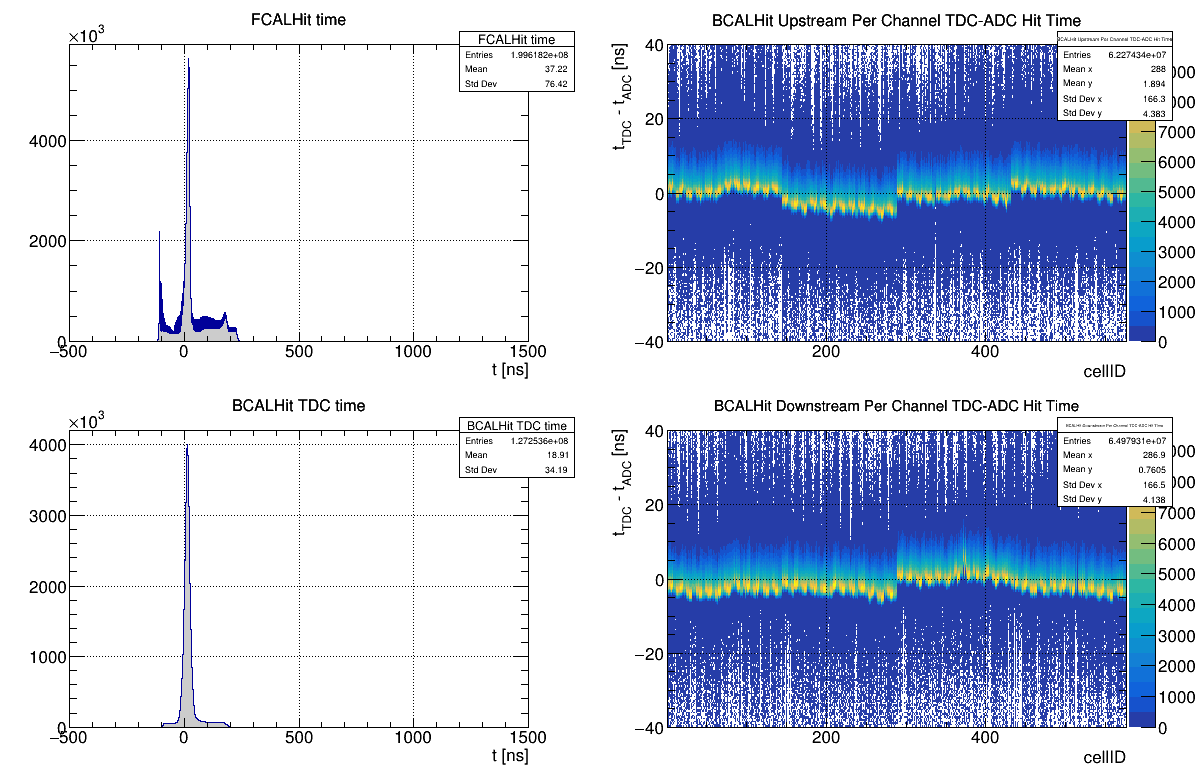
- Calorimeter Timing - The right two plots aren't aligned at zero because not all corrections are currently applied. If there is a 32 ns shift in part of this data, please note this.
- Drift Chamber Timing - In each case, the main peaks should line up at zero, but often have other structures. Ignore the first few bins of the lower left plot (they mostly say something about the noise in the detector). There can be 32 ns shifts in the lower right plot.
- PID System Timing - Nothing to note yet.
- Tagger Timing - The signal to background levels of the left two plots depend on the electron beam current.
- Track Matched Timing - Some overlap here with the tracking timing. The new plots should be centered at zero.
- Tagger/RF Timing - Look for the nice "picket fences" on the right two plots, and that in the bottom left plot each channel peaks at zero.
- Tagger/SC Timing - Should be similar to Tagger/RF Timing but with larger resolution.
Analysis
- Tracking 1 - [ link ]
- Tracking 3 - [ link ]
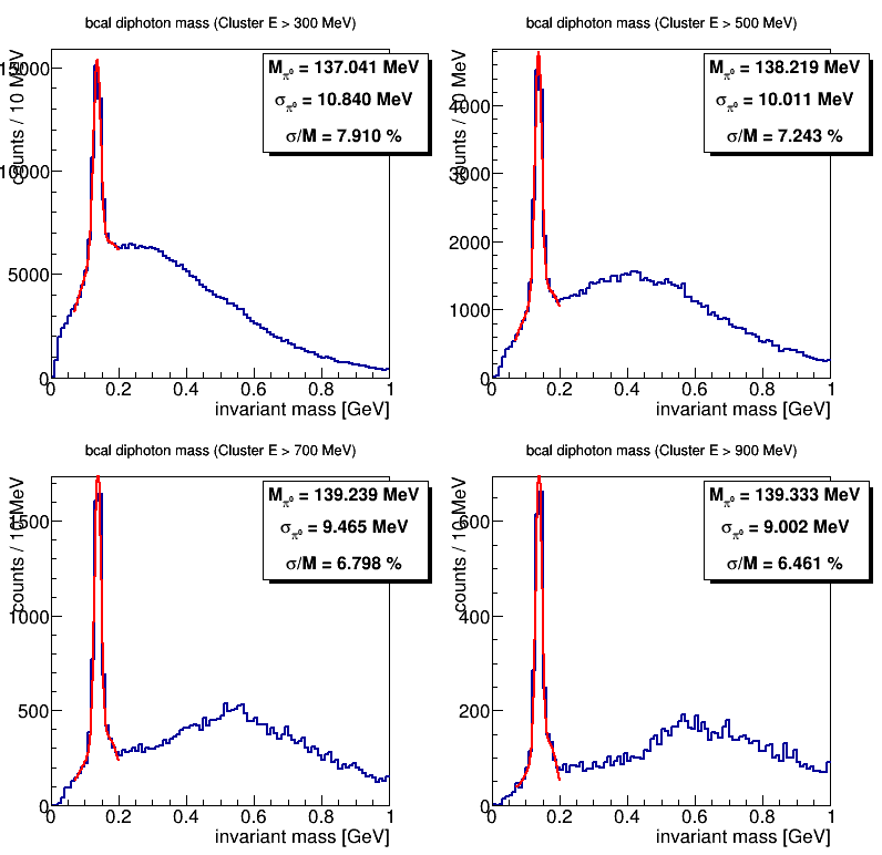
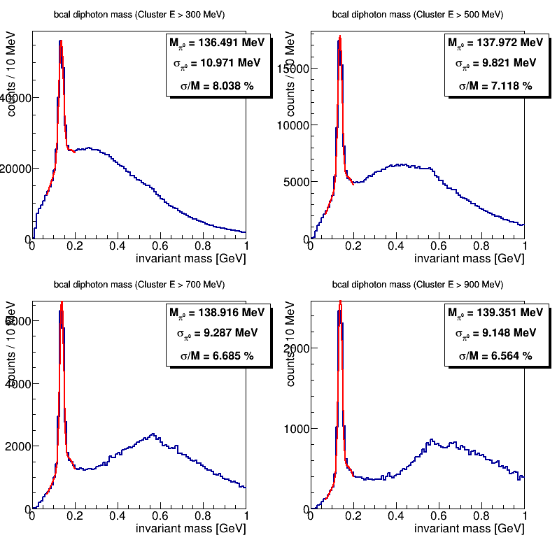
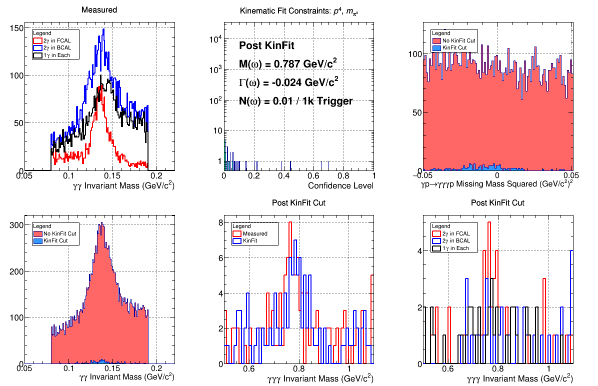
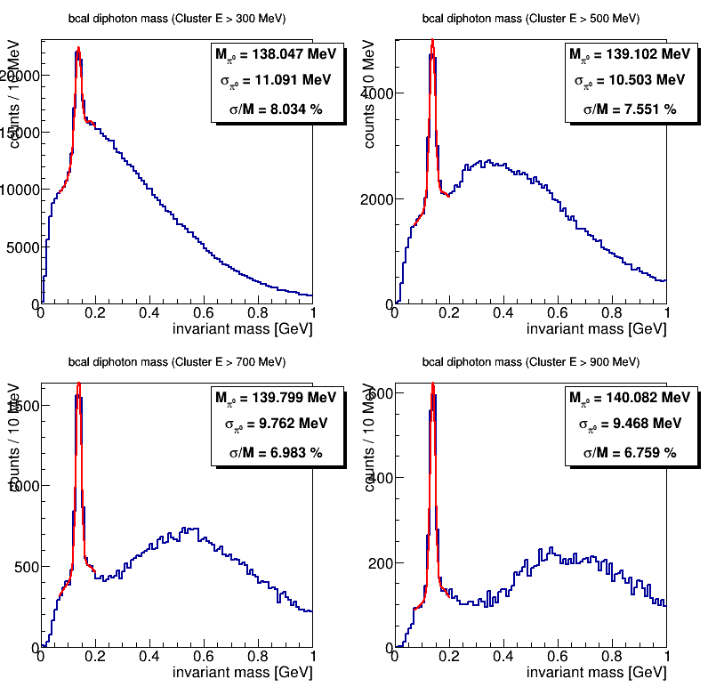
- Check BCAL pi0 - Reference: [ link ]
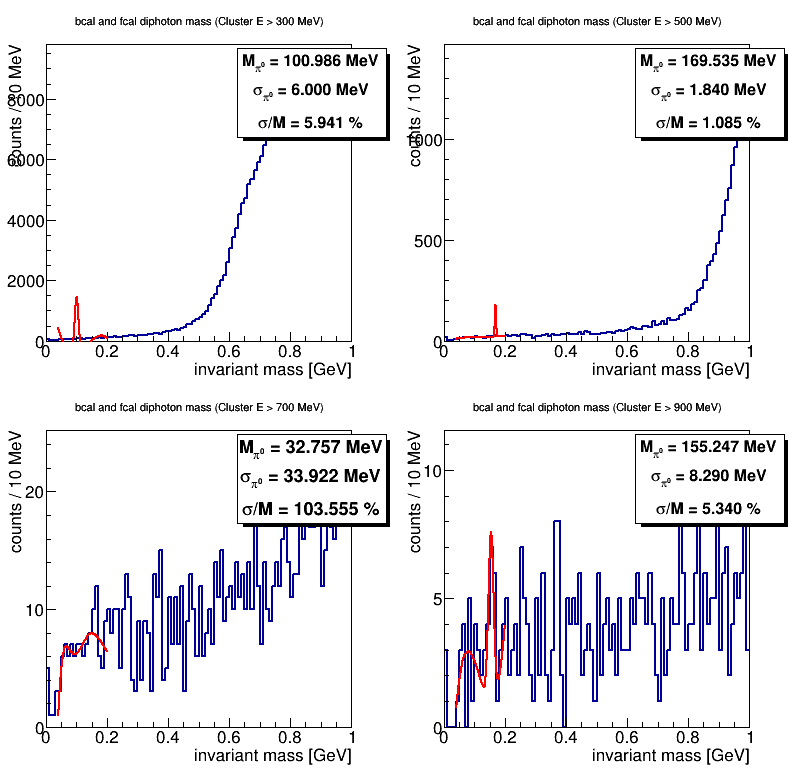
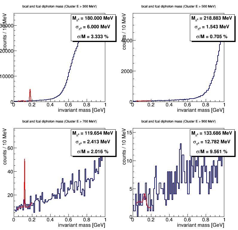
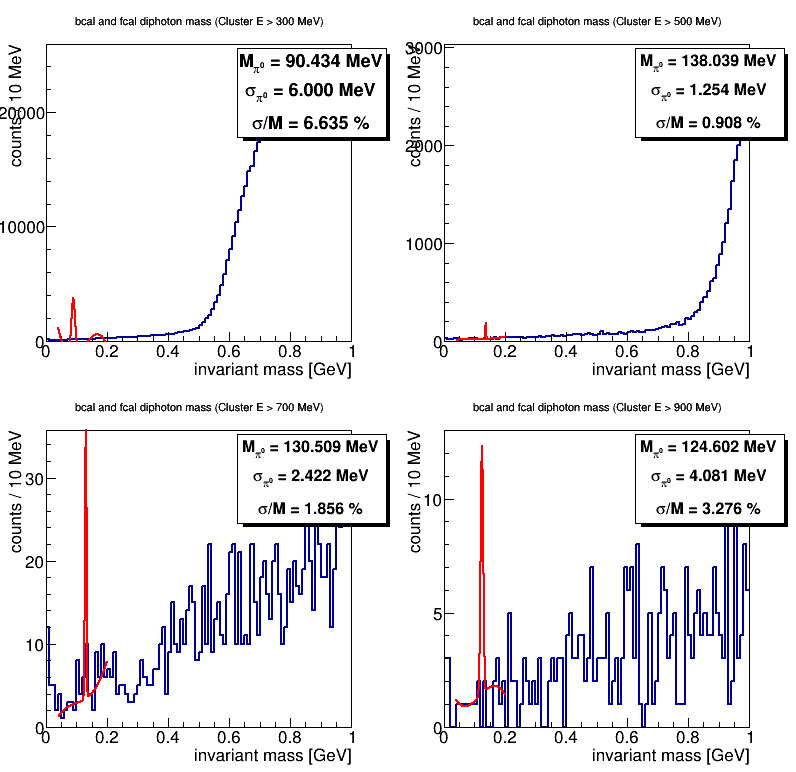
- Check BCAL/FCAL pi0 - Reference: [ link ]
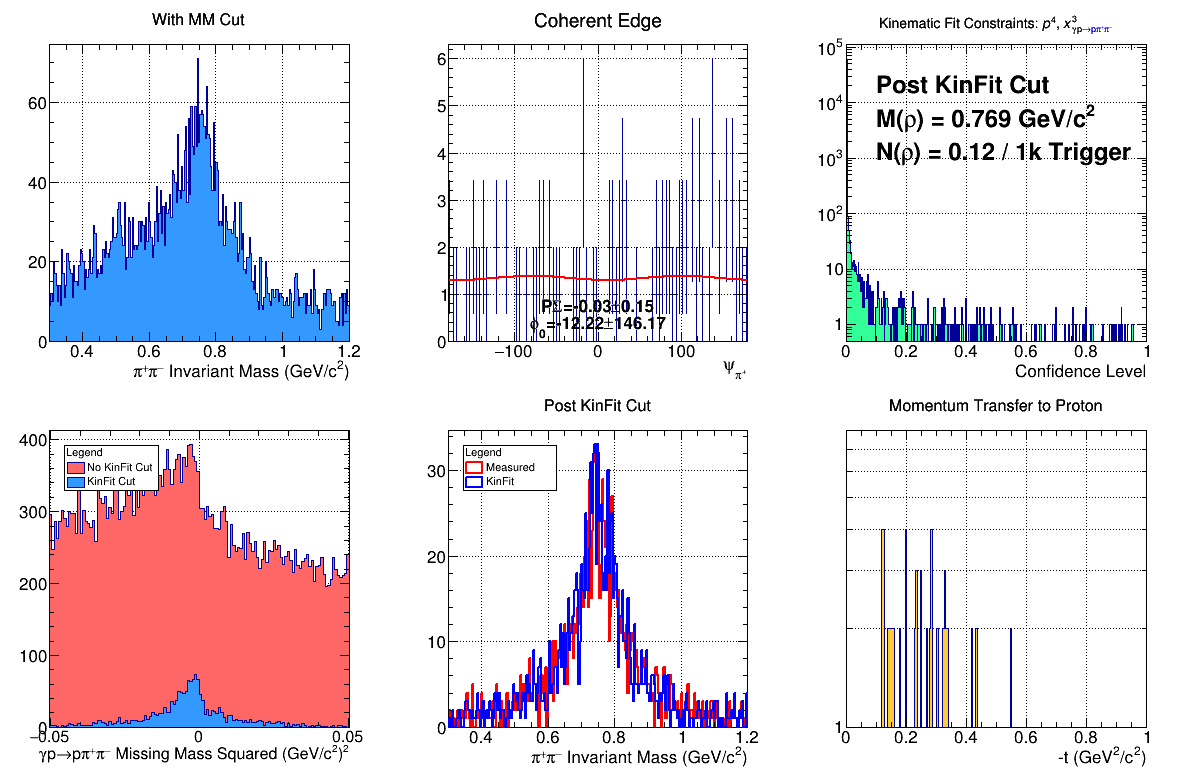
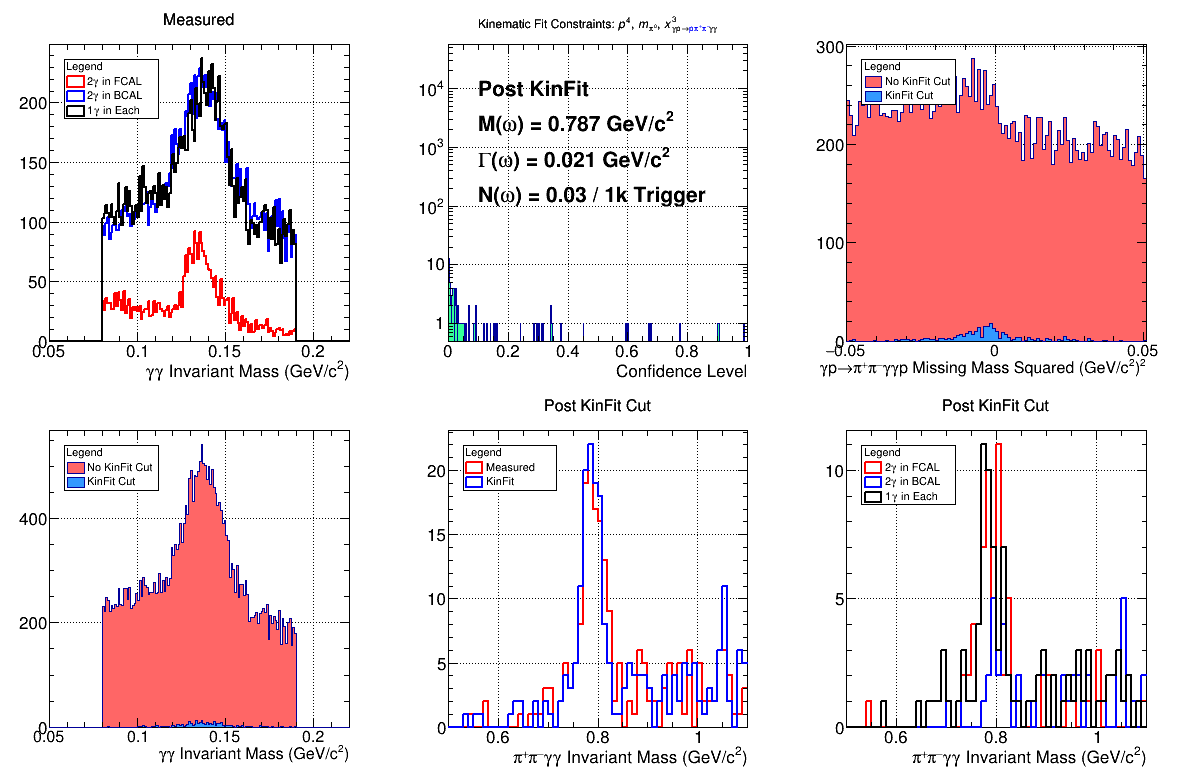
- Check p+2pi - Reference: [ link ]
- Check p+3pi - Reference: [ link ]
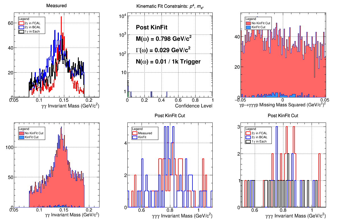
- Check p+pi0g - Reference: [ link ]
Analysis Reference Plots
Beryllium Target
![]()
![]()


Full Liquid Helium Target
![]()
![]()
Empty Liquid Helium Target
![]()
![]()
Analysis Notes
Generally in these plots, there will be a difference between diamond and amorphous radiator running. Should probably add some references for non-diamond plots.
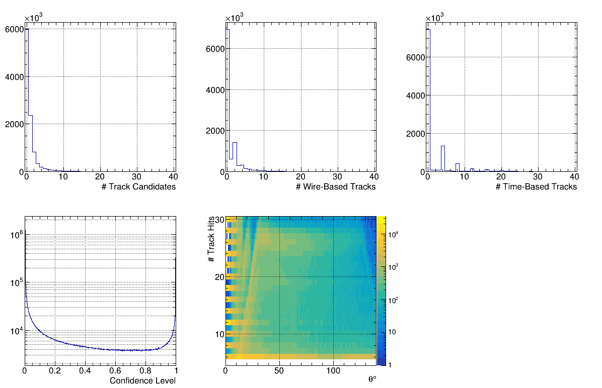
- Tracking 1 - There should be some mild dependence on beam current and radiator. Note the spikes in the upper right plot are because we have 4 hypotheses fit to a track by default. The lower left plot does have a peak at zero.
- Tracking 3 -
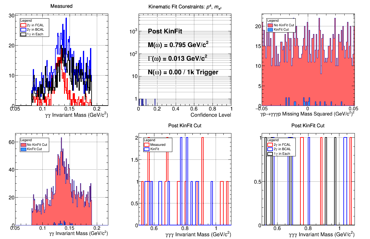
- Check BCAL pi0 - The fitted peak should near at the correct pi0 mass of 135 MeV.
- Check BCAL/FCAL pi0 - The fitted peak should be lower than the correct pi0 mass, I think because the wrong vertex is used.
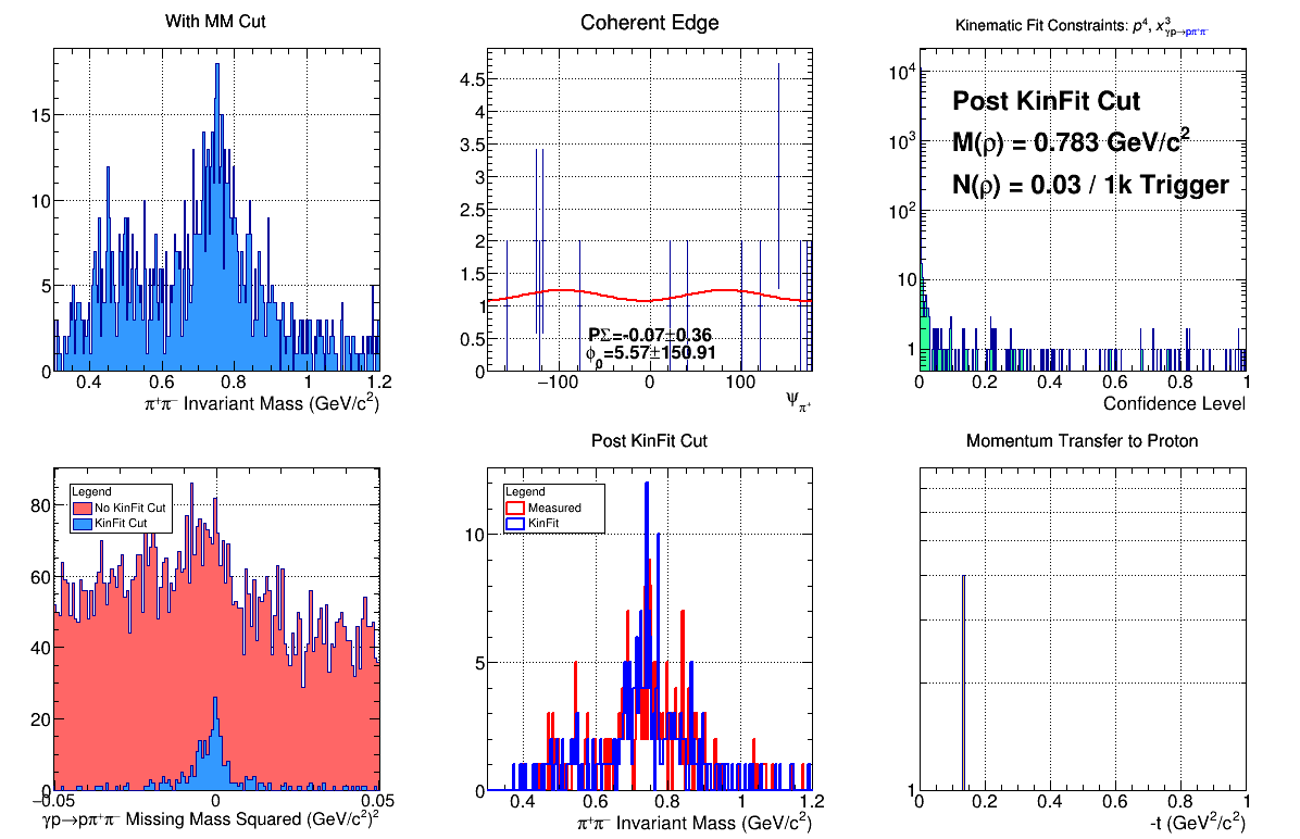
- Check p+2pi - The top middle plot should have a sin(2phi) shape for diamond runs. Note that the yields in the top right plot vary from run to run on the order of 10-20%.
- Check p+3pi -Note that the yields in the top right plot vary from run to run on the order of 10-20%.
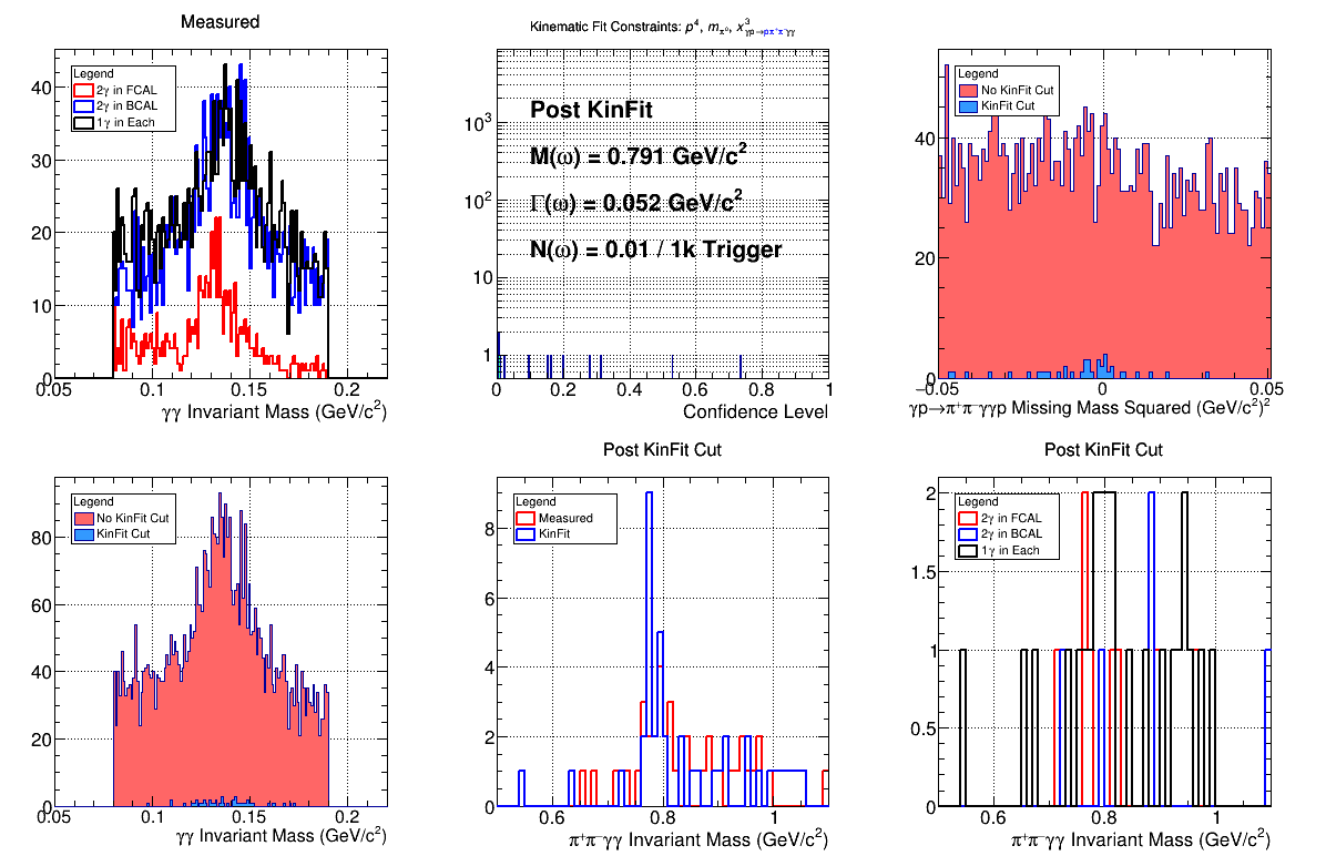
- Check p+pi0g - Note that the yields in the top right plot vary from run to run on the order of 10-20%.
- Note that these yields are sensitive to the tagger range used! This changes for different beam current settings.