Difference between revisions of "BCal Beam Test Plots, May 8, 2007"
(→Mean Time Resolution σ<sub>T</sub>) |
(→Time Difference Resolution σ<sub>ΔT</sub>) |
||
| Line 29: | Line 29: | ||
[[Image:Test a 7 8 9 0b.gif|360px]] | [[Image:Test a 7 8 9 0b.gif|360px]] | ||
[[Image:Timedifres.gif|360px]] | [[Image:Timedifres.gif|360px]] | ||
| + | |||
| + | The bottom left image is the distribution before walk correction (black) and after walk correction (red). The bottom right image are the means of the left two plots. Notice that there are little or no fluctuations now that the tagger is not involved. | ||
Revision as of 16:40, 7 May 2007
Energy Weighting
The timing resolution of the BCal should improve when one begins to group the individual cells into a cluster of cells. Ideally one would like to weight each cell by its own resolution (i.e. multiply by the inverse squared) such that cells with a poorer resolution contribute less to the overall resolution. However, one also needs to know the resolution for each cell to a good degree otherwise the cells which truly have a lower resolution might end up contributing more than they should giving one a worse resolution overall as a result. The next best thing would be to weight each cell by its deposited energy which is directly measured. The ADC signal is proportional to the energy deposit by some calibration constant. The inverse square of the resolution of the cell is also proportional to the energy deposited. Hence, we define the time at each calorimeter end to be
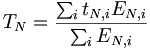
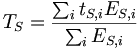
and the average of TN and TS defines the mean time. Each end of the cell should have identical responses and we can assume EN = ES. For the case where the beam is at dead center of the module the ADC signals should also be similar except for some gain correction factors. We can then define the mean time and time difference as
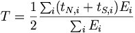
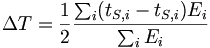
respectively. We estimate the contribution to the resolution from jitter in the Master OR signal from the Tagger to be σtagger = 113 ps which should be subtracted in quadrature from the constant term of the fit of the mean time resolution to obtain the correct mean time resolution. ΔT and T are the difference and sum of TN and TS and therefore the distributions have the same rms. spread. One therefore expects σT = σΔT.
Mean Time Resolution σT


The bottom left image is the distribution before walk correction (black) and after walk correction (red). The bottom right image are the means of the left two plots. Notice the large fluctuations even after walk corrections.
Time Difference Resolution σΔT


The bottom left image is the distribution before walk correction (black) and after walk correction (red). The bottom right image are the means of the left two plots. Notice that there are little or no fluctuations now that the tagger is not involved.