Difference between revisions of "February 17, 2009 Physics"
From GlueXWiki
m (Text replacement - "http://argus.phys.uregina.ca/gluex" to "https://halldweb.jlab.org") |
|||
| (4 intermediate revisions by 2 users not shown) | |||
| Line 1: | Line 1: | ||
| + | == Calibration == | ||
| + | |||
* Reconstructed Z minus generated Z over the length of the module. The deviations are less than 0.5 cm. | * Reconstructed Z minus generated Z over the length of the module. The deviations are less than 0.5 cm. | ||
[[Image:MeanrecZ minus genZ.png|400px]] | [[Image:MeanrecZ minus genZ.png|400px]] | ||
| − | * Reconstructed single photon energy '''BEFORE corrections''' | + | * Reconstructed single photon (0 to 4 GeV) energy '''BEFORE corrections''' |
| + | A flat correction has been made for sampling fraction and smearing has been applied in DBCALMCResponse. The threshold is a flat 6 MeV/segment. | ||
[[Image:RecEgenE vs recZ.png|400px]] [[Image:RecEgenE vs recZ mean.png|400px]] | [[Image:RecEgenE vs recZ.png|400px]] [[Image:RecEgenE vs recZ mean.png|400px]] | ||
| Line 9: | Line 12: | ||
| − | * Reconstructed single photon energy '''AFTER corrections''' | + | * Fit function for reconstructed energy for slices of z along the BCAL |
| + | |||
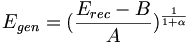
| + | <math>\frac{E_{rec}}{E_{gen}} = A*E_{gen}^{\alpha}+B/E_{gen} </math> | ||
| + | |||
| + | so that | ||
| + | |||
| + | <math>E_{gen} = (\frac{ E_{rec} - B }{A})^{\frac{1}{1+\alpha}} </math> | ||
| + | |||
| + | [[Image:H31 1 sum nCellLT5.png|400px]] | ||
| + | |||
| + | |||
| + | |||
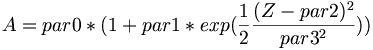
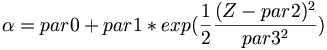
| + | * Fit function for parameter A, \alpha, and B | ||
| + | |||
| + | |||
| + | <math> A = par0 * ( 1 + par1 * exp(\frac{1}{2}\frac{(Z-par2)^{2}}{par3^{2}})) </math> | ||
| + | <math> \alpha = par0 + par1 * exp(\frac{1}{2}\frac{(Z-par2)^{2}}{par3^{2}}) </math> | ||
| + | <math> B = par0 + par1 * exp(\frac{1}{2}\frac{(Z-par2)^{2}}{par3^{2}}) </math> | ||
| + | |||
| + | [[Image:Fit par1 sum nCellLT5.png|300px| "A"]] [[Image:Fit par2 sum nCellLT5.png|300px|"\alpha"]] [[Image:Fit par3 sum nCellLT5.png|300px|"B"]] | ||
| + | |||
| + | |||
| + | |||
| + | |||
| + | == Reconstruction == | ||
| + | |||
| + | * Reconstructed single photon (0 to 4 GeV) energy '''AFTER corrections''' | ||
[[Image:EPhogenE vs recZ.png|400px]] [[Image:EPhogenE vs recZ mean.png|400px]] | [[Image:EPhogenE vs recZ.png|400px]] [[Image:EPhogenE vs recZ mean.png|400px]] | ||
| − | * Unconstrained invariant mass (left) and fit confidence level (right) for '''pi0''' candidates after the mass-constrained kinematic fit. Candidates with Chi2 < 3(5) are shown in red (blue). These are from decays of a2(1320)to eta-pi0 to 4 gamma generated in genr8. This can be compared with Figure 5.12 in [ | + | * Unconstrained invariant mass (left) and fit confidence level (right) for '''pi0''' candidates after the mass-constrained kinematic fit. Candidates with Chi2 < 3(5) are shown in red (blue). These are from decays of a2(1320)to eta-pi0 to 4 gamma generated in genr8. The protons have been suppressed. This can be compared with Figure 5.12 in [https://halldweb.jlab.org/DocDB/0009/000989/001/simulation.pdf Calorimeter physics simulations and reconstruction for the Calorimetry Review (GlueX Portal)] |
[[Image:Figure512.png]] | [[Image:Figure512.png]] | ||
| Line 20: | Line 49: | ||
| − | * Unconstrained invariant mass (left) and fit confidence level (right) for '''eta''' candidates after the mass-constrained kinematic fit. Candidates with Chi2 < 3(5) are shown in red (blue). These are from decays of a2(1320)to eta-pi0 to 4 gamma generated in genr8.This can be compared with Figure 5.13 in [ | + | * Unconstrained invariant mass (left) and fit confidence level (right) for '''eta''' candidates after the mass-constrained kinematic fit. Candidates with Chi2 < 3(5) are shown in red (blue). These are from decays of a2(1320)to eta-pi0 to 4 gamma generated in genr8. The protons have been suppressed. This can be compared with Figure 5.13 in [https://halldweb.jlab.org/DocDB/0009/000989/001/simulation.pdf Calorimeter physics simulations and reconstruction for the Calorimetry Review (GlueX Portal)] |
[[Image:Figure513.png]] | [[Image:Figure513.png]] | ||
| + | |||
| + | * | ||
| + | == Semi-parametric Monte Carlo == | ||
| + | Here are [[Media:20090217_hdparsim_photon.pdf|some slides]] David showed at this meeting. | ||
| + | |||
| + | |||
| + | == Thoughts, to do list, etc. from meeting == | ||
| + | Z.P., B.L., D.L., M.S., R.M. | ||
| + | |||
| + | 1. look at difference between reconstructed and generated z position for less than 65 cm | ||
| + | 2. look at single photon reconstruction efficiencies | ||
| + | 3. adjust the error matrix for the BCAL (look in PID/DPhoton_factory.cc) | ||
| + | |||
| + | Next Steps: | ||
| + | 1. look at the a2 mass peak - adjust cuts on the eta and pi0 masses | ||
| + | 2. introduce Pythia background - skim off the wanted events by cutting on the total neutral energy (but we need to record the total number of events before skimming) - hd_filter is a good program example | ||
| + | 3. cut on eta and pi0 masses, then look at the effect on the different angular distributions (i.e. Gottfried-Jackson angles, etc.) | ||
Latest revision as of 12:40, 14 March 2017
Contents
Calibration
- Reconstructed Z minus generated Z over the length of the module. The deviations are less than 0.5 cm.

- Reconstructed single photon (0 to 4 GeV) energy BEFORE corrections
A flat correction has been made for sampling fraction and smearing has been applied in DBCALMCResponse. The threshold is a flat 6 MeV/segment.


- Fit function for reconstructed energy for slices of z along the BCAL
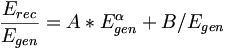
so that

- Fit function for parameter A, \alpha, and B


Reconstruction
- Reconstructed single photon (0 to 4 GeV) energy AFTER corrections


- Unconstrained invariant mass (left) and fit confidence level (right) for pi0 candidates after the mass-constrained kinematic fit. Candidates with Chi2 < 3(5) are shown in red (blue). These are from decays of a2(1320)to eta-pi0 to 4 gamma generated in genr8. The protons have been suppressed. This can be compared with Figure 5.12 in Calorimeter physics simulations and reconstruction for the Calorimetry Review (GlueX Portal)

- Unconstrained invariant mass (left) and fit confidence level (right) for eta candidates after the mass-constrained kinematic fit. Candidates with Chi2 < 3(5) are shown in red (blue). These are from decays of a2(1320)to eta-pi0 to 4 gamma generated in genr8. The protons have been suppressed. This can be compared with Figure 5.13 in Calorimeter physics simulations and reconstruction for the Calorimetry Review (GlueX Portal)

Semi-parametric Monte Carlo
Here are some slides David showed at this meeting.
Thoughts, to do list, etc. from meeting
Z.P., B.L., D.L., M.S., R.M.
1. look at difference between reconstructed and generated z position for less than 65 cm
2. look at single photon reconstruction efficiencies
3. adjust the error matrix for the BCAL (look in PID/DPhoton_factory.cc)
Next Steps:
1. look at the a2 mass peak - adjust cuts on the eta and pi0 masses
2. introduce Pythia background - skim off the wanted events by cutting on the total neutral energy (but we need to record the total number of events before skimming) - hd_filter is a good program example
3. cut on eta and pi0 masses, then look at the effect on the different angular distributions (i.e. Gottfried-Jackson angles, etc.)