Difference between revisions of "HOWTO Analyze a FDC Flatness Scan"
(Incomplete first draft) |
(Added photos of granite slab) |
||
| Line 20: | Line 20: | ||
= Interpreting the Scan Data = | = Interpreting the Scan Data = | ||
| + | {| | ||
| + | | | ||
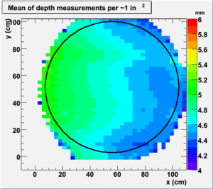
[[Image:20081120_fdc_mean_cathode.gif|thumb|right|Example of the mean value of a cathode plane from scan "plane004 000deg 2008_11_06 09_26_26"]] | [[Image:20081120_fdc_mean_cathode.gif|thumb|right|Example of the mean value of a cathode plane from scan "plane004 000deg 2008_11_06 09_26_26"]] | ||
| Line 29: | Line 31: | ||
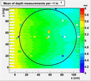
The mounting rails for the laser itself are not perfectly straight. This is evidenced by a noticeable and similar "wave" in both the cathode scan and a scan of the granite slab itself. The image on the right shows the means of a scan of a cathode plane while the image on the left shows the same thing, but for the granite slab itself. | The mounting rails for the laser itself are not perfectly straight. This is evidenced by a noticeable and similar "wave" in both the cathode scan and a scan of the granite slab itself. The image on the right shows the means of a scan of a cathode plane while the image on the left shows the same thing, but for the granite slab itself. | ||
| + | |- | ||
| + | | | ||
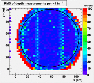
| + | [[Image:20081120_fdc_rms_cathode.gif|thumb|right|Example of the mean value of a cathode plane from scan "plane004 000deg 2008_11_06 09_26_26"]] | ||
| + | |||
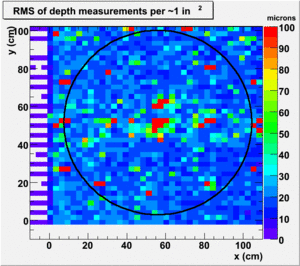
| + | [[Image:20081120_fdc_rms_granite.gif|thumb|left|Example of the mean value of the granite slab from scan "plane999 999deg 2008_11_06 08_51_09"]] | ||
| + | |||
| + | The RMS values for the cathode and granite scans are shown here on the right and left respectively. These correspond to the same bins used for the plots above of the means. In the cathode scan on the right, the 2 tape lines are easily seen while on the left, several drill holes in the granite slab show up as red spots. The color scales go from 0 to 100 microns so blue colors have an RMS of around 30 microns or less. Green is in the 50-60 micron range while red is in the 100 or more micron range. | ||
| + | |||
| + | |- | ||
| + | | | ||
[[Image:20081120_cathode_granite.gif|thumb|right|Cathode (red) and granite (black) scans from scan "plane004 000deg 2008_11_06 09_26_26" and "plane999 999deg 2008_11_06 08_51_09" respectively]] | [[Image:20081120_cathode_granite.gif|thumb|right|Cathode (red) and granite (black) scans from scan "plane004 000deg 2008_11_06 09_26_26" and "plane999 999deg 2008_11_06 08_51_09" respectively]] | ||
| Line 34: | Line 46: | ||
| − | + | |} | |
| − | + | <hr> | |
| − | + | One interesting thing to note is the imperfections in both the ''mean'' and the ''rms'' of the scan of the granite slab above. These correspond to drilled holes and divots in the slab's surface as shown in the 2 plots below. The image on the left is a photo of the granite slab and the one on the right is the same, but with the ''mean'' plot from the scan data overlayed. | |
| + | {| | ||
| + | | [[Image:20081120_granite_slab.jpg | 300px]] | ||
| + | | [[Image:20081120_granite_plot_overlay.jpg | 300 px]] | ||
| + | |} | ||
= Location of the code = | = Location of the code = | ||
Revision as of 14:18, 20 November 2008
Quick Start
- To get started you need a scan data file. These have names like "plane004 000deg 2008_11_06 09_26_26.txt" These are generally found in the ??? directory on the Linux computer kept in EEL126 next to the FDC laser scanner. Note that this computer is not connected to the outside network so if the analysis is being done on a different computer, the file will need to be copied via a USB drive.
- Run the snake_mktree program giving the data file as the only argument.
- e.g. snake_mktree plane004 000deg 2008_11_06 09_26_26.txt"
- Note here that the double quotes(") surrounding the file name are needed since the filename contains spaces.
- The program should create a ROOT file with the same name as the input file, only with a ".root" suffix.
- Run the ROOT macros fdc_mean.C and fdc_rms.C on the resulting root file.
- e.g.
- root -q -b 'fdc_mean.C("plane004 000deg 2008_11_06 09_26_26.root")'
- root -q -b 'fdc_rms.C("plane004 000deg 2008_11_06 09_26_26.root")'
- Notice the single quotes around the ''fdc_rms.C("plane004 000deg 2008_11_06 09_26_26.root". These are because the
- shell will try interpreting the parenthesis while we really want them to be passed as part of the argument.
- These should create the files fdc_mean.gif and fdc_rms.gif respectively.
Interpreting the Scan Data
|
The mounting rails for the laser itself are not perfectly straight. This is evidenced by a noticeable and similar "wave" in both the cathode scan and a scan of the granite slab itself. The image on the right shows the means of a scan of a cathode plane while the image on the left shows the same thing, but for the granite slab itself. |
|
The RMS values for the cathode and granite scans are shown here on the right and left respectively. These correspond to the same bins used for the plots above of the means. In the cathode scan on the right, the 2 tape lines are easily seen while on the left, several drill holes in the granite slab show up as red spots. The color scales go from 0 to 100 microns so blue colors have an RMS of around 30 microns or less. Green is in the 50-60 micron range while red is in the 100 or more micron range. |
|
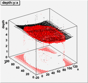
The animation on the right shows another view of these two scans on the same plot to further illustrate the similarity in the "wave" indicating it is the scanner and not the scannee that is the source.
|
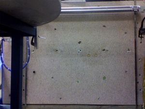
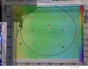
One interesting thing to note is the imperfections in both the mean and the rms of the scan of the granite slab above. These correspond to drilled holes and divots in the slab's surface as shown in the 2 plots below. The image on the left is a photo of the granite slab and the one on the right is the same, but with the mean plot from the scan data overlayed.
|
|
Location of the code
The source code for all of the laser scanner system is kept in the Hall-D subversion repository in the following directory:
