Kuraray Fibre Tests
Contents
Detector Setup
- The fibre is cut and polished on both ends with the Fiber Fin polisher (the label must be removed due to its placement too close to the end)
- The far end of the fibre is painted black with an enamel paint (used for painting scale models).
- The fibre is placed in a 4m x 1mm groove in a black poly-ethylene bar ("puck board")
- The unpainted end is inserted into and held in place by a bare-fibre SMA-connector from Ocean Optics.
- A UV LED (380nm) is used to illuminate the fibre from above, and perpendicularly to the fiber's long axis
- The spectra are obtained using an Ocean Optics spectrophotometer
Fibre Spectra
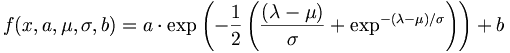
Typical fibre spectra at 10,100 and 300 cm.The green data points are the raw spectra as seen by the photo-spectrometer. The light blue points are scaled by an approximation to the quantum efficiency of a Bi-Alkali photocathode. The fit functions were of double Moyal type (see equation below). The reader is directed to the Regina Fiber NIM paper for details. The fits were cross checked versus simply summing the bins (~0.3nm) resulting from the grating in the Ocean Optics spectrophotometer.


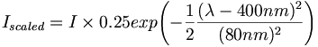
Bi-Alkali Quantum efficiency approximation

Attenuation lengths
- The attenuation length is found by taking the integral of the fit function of the scaled spectra and fitting that as a function of distance from the spectrometer. The fit function is a single exponential: I = A * exp(-x/B). The attenuation length is then effectively that of the fibre as seen by a PMT.
So far 6 fibers have had their attenuation lengths measured:
Attenuation length:
| Blake | Andrei | Kuraray | |||
|---|---|---|---|---|---|
| fibre # |  |
 |
|
|
|
| 01-3 | 440 | 13 | 442.3 | 8.7 | 368.0 |
| 02-3 | 435 | 12 | |||
| 04-3 | 428 | 6 | |||
| 05-3 | 417 | 9 | |||
| 07-3 | 464 | 8 | |||
| 09-3 | 448 | 11 | |||
| 23-2 | 443 | 10 | 445.6 | 9.0 | 369.1 |
| 26-2 | 478 | 9 | 477.1 | 9.6 | 374.8 |
| 32-2 | 414 | 30 | 451.5 | 9.6 | 377.5 |
| 33-2 | 398 | 15 | 409.4 | 7.3 | 385.4 |
| 49-3 | 441 | 12 | 443.5 | 8.8 | 377.4 |
| Avg | 437 |  |

- Reproducing the results
The following two measurements were taken of the same fibre, the first was the afternoon previous to the second measurement, re-coupling it before the second measurement. You can notice that similar features show up in the measurements, and which do not appear in other attenuation spectra, that indicates that there are features within the fibre smaller than 10cm that affect the light output at that point on the fibre. This may be a crack in the core of the fibre or possibly a change in the doping in that region or stresses in the polystyrene due to the extrusion process. This also indicates that the measuring process is stable and repeatable within coupling tolerances.


*note that the horizontal axis is labeled incorrectly as wavelength. This should be position(cm).
- April 2nd Update
The correction function used to simulate the bi-alkali readout was modified to that as shown on Kuraray's web page for the PMT used in their attenuation length measurements. The scaling function is now
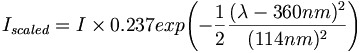
This has the result of increasing the attenuation length by approximately 2.5% over what was shown previously. However, the attenuation length measured with the spectrometer is still 70-80 cm longer than what Kuraray measured.
| Blake | ||
|---|---|---|
| fibre # |  |

|
| 01-3 | 454 | 14 |
| 02-3 | 448 | 12 |
| 04-3 | 438 | 6 |
| 05-3 | 428 | 9 |
| 07-3 | 478 | 9 |
| 09-3 | 462 | 12 |
| 23-2 | 459 | 11 |
| 26-2 | 495 | 10 |
| 32-2 | 426 | 32 |
| 33-2 | 409 | 16 |
| 48-3 | 444 | 8 |
| 49-3 | 454 | 13 |
| 53-3 | 481 | 11 |
| Avg | 452 |
|
- Andrei's plots
Andrei used the same data but his own analysis scripts. The integrals are found by summing the bins instead of finding the integral of the fit function as in Blake's analysis. Blake had also checked his fitting function (Moyal) versus bin-summing and the results were consistent.


Initial Conclusions
- The Kuraray numbers from the same fibres, over the same integrated range (100-285cm), show lower (more conservative?) values for the attenuation length. One source of difference can be the PMT assumptions we have made.
- The Specifications for the Scintillating Fibres required that "The bulk attenuation length of a bare fiber shall exceed 350cm, while the effective attenuation length of the fiber shall exceed 300cm measured with a bialkali photomultiplier tube. The RMS variation in attenuation length shall be less than 10% throughout the fiber lots." This seems to be the case.
Future Tasks
- Extract bare fibre attenuation length
- A few cross checks
- The goal is to measure 25 fibres in the next few days
- Make a few slight modifications to the measuring apparatus (i.e larger diffuse UV beam)
- There's always something...