Difference between revisions of "Kuraray Fibre Tests"
From GlueXWiki
| Line 1: | Line 1: | ||
==Detector Setup== | ==Detector Setup== | ||
| − | #The fibre is cut and polished on both ends with the Fiber Fin polisher (the label must be removed due to it's placement too close to the end) | + | #The fibre is cut and polished on both ends with the [http://www.fiberfin.com/products/more/FF-FF4.htm Fiber Fin] polisher (the label must be removed due to it's placement too close to the end) |
#The far end of the fibre is painted black with an enamel paint (used for painting scale models). | #The far end of the fibre is painted black with an enamel paint (used for painting scale models). | ||
| − | #The fibre is placed in a 4m | + | #The fibre is placed in a 4m x 1mm groove in a black poly-ethylene bar ("puck plastic") |
| − | #The unpainted end is inserted into and held in place by a [ http://www.oceanoptics.com/products/fiberkits.asp#adapter bare-fibre SMA-connector] from Ocean Optics. | + | #The unpainted end is inserted into and held in place by a [http://www.oceanoptics.com/products/fiberkits.asp#adapter bare-fibre SMA-connector] from Ocean Optics. |
#A UV LED (380nm) is used to illuminate the fibre from above | #A UV LED (380nm) is used to illuminate the fibre from above | ||
#The spectra are obtained using an [http://www.oceanoptics.com/products/usb4000.asp Ocean Optics photo-spectrometer] | #The spectra are obtained using an [http://www.oceanoptics.com/products/usb4000.asp Ocean Optics photo-spectrometer] | ||
| + | |||
| + | |||
== Fibre Spectra == | == Fibre Spectra == | ||
| Line 14: | Line 16: | ||
[[Image:K49-3-cl-blk-000.png |250px|"10cm"]][[Image:K49-3-cl-blk-009.png |250px|"100cm"]][[Image:K49-3-cl-blk-029.png |250px|"300cm"]] | [[Image:K49-3-cl-blk-000.png |250px|"10cm"]][[Image:K49-3-cl-blk-009.png |250px|"100cm"]][[Image:K49-3-cl-blk-029.png |250px|"300cm"]] | ||
| − | ==Bi- | + | ==Bi-Alkali Quantum efficiency approximation== |
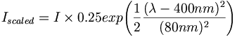
<math>I_{scaled} = I \times 0.25 exp{\left(\frac{1}{2}\frac{(\lambda-400nm)^{2}}{(80nm)^{2}}\right) } </math> | <math>I_{scaled} = I \times 0.25 exp{\left(\frac{1}{2}\frac{(\lambda-400nm)^{2}}{(80nm)^{2}}\right) } </math> | ||
[[Image:Quantumefficiency.png|250px]] | [[Image:Quantumefficiency.png|250px]] | ||
| + | |||
| + | |||
| + | ==Attenuation lengths== | ||
| + | |||
| + | #The attenuation length is found by taking the integral of the fit function of the ''scaled spectra'' and fitting that as a function of distance from the spectrometer. The fit function is a single exponential: I = A * exp(-x/B). The attenuation length is then effectively that of the fibre as seen by a PMT. | ||
| + | |||
| + | So far 6 fibers have had their attenuation lengths measured: | ||
| + | |||
| + | '''Attenuation length:''' | ||
| + | {| class="wikitable" style="text-align:center; border="1" | ||
| + | !fibre # !! <math>\lambda</math> !! <math>d\lambda</math> | ||
| + | |- | ||
| + | ! 01-3 || 440 || 12 | ||
| + | |- | ||
| + | ! 23-2 || 443 || 10 | ||
| + | |- | ||
| + | ! 26-2 || 478 || 10 | ||
| + | |- | ||
| + | ! 32-2 || 414 || 30 | ||
| + | |- | ||
| + | ! 33-2 || 398 || 15 | ||
| + | |- | ||
| + | ! 49-3 || 441 || 12 | ||
| + | |- | ||
| + | ! Avg || 436 || 15 | ||
| + | |} | ||
| + | [[Image:Attenuation 6spectra.png|400px]] | ||
Revision as of 20:20, 18 March 2009
Contents
Detector Setup
- The fibre is cut and polished on both ends with the Fiber Fin polisher (the label must be removed due to it's placement too close to the end)
- The far end of the fibre is painted black with an enamel paint (used for painting scale models).
- The fibre is placed in a 4m x 1mm groove in a black poly-ethylene bar ("puck plastic")
- The unpainted end is inserted into and held in place by a bare-fibre SMA-connector from Ocean Optics.
- A UV LED (380nm) is used to illuminate the fibre from above
- The spectra are obtained using an Ocean Optics photo-spectrometer
Fibre Spectra
Typical fibre spectra at 10,100 and 300 cm.The green data points are the raw spectra as seen by the photo-spectrometer. The light blue points are scaled by an approximation to the quantum efficiency of a Bi-Alkali photocathode.


Bi-Alkali Quantum efficiency approximation

Attenuation lengths
- The attenuation length is found by taking the integral of the fit function of the scaled spectra and fitting that as a function of distance from the spectrometer. The fit function is a single exponential: I = A * exp(-x/B). The attenuation length is then effectively that of the fibre as seen by a PMT.
So far 6 fibers have had their attenuation lengths measured:
Attenuation length:
| fibre # |  |

|
|---|---|---|
| 01-3 | 440 | 12 |
| 23-2 | 443 | 10 |
| 26-2 | 478 | 10 |
| 32-2 | 414 | 30 |
| 33-2 | 398 | 15 |
| 49-3 | 441 | 12 |
| Avg | 436 | 15 |
