Regina Group Meeting, October 26, 2006

Attendees: George, Blake, Yianna, Zisis (Regina) - Christine's (Athens) input was received by phone the day before

1. Regina Analysis: following the teleconference of October 23, this meeting was held to discuss details of the Regina analysis.
   • Runs to focus on initially: The data will be examined initially for the normal (90 degree) vertical scan runs (No. 2319, 2322, 2323, 2324, 2332, 2333, 2334) since the collection of these runs dumps energy not only in the middle sector but also in the top and bottom ones.
   • Monte Carlo: the MC will be run using tha tagged photon spectrum from the data as a sampling spectrum for GEANT. Blake's code creates histos for viewing spectral shapes and ntuples for applying cuts and doing analysis. (In the future we will convert this to root trees).
   • Analysis Procedure:
     1. Extract the spectral shapes and means from the energy deposited per cell from the MC for photons. Form ratios of the means of all cells using cell #8 as unity.
     2. Apply 'clean up' cuts to the data (e.g. photon=1), and plot ADC per cell versus its MC energy mean to extract the ADC->MeV calibration.
     3. Use a suitable spectrum for cosmics and add this (low energy deposited) point to the calibration procedure.
     4. After the calibration form the North and South sums. Form the geometric mean 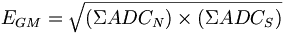$E_{{GM}}={\sqrt {(\Sigma ADC_{N})\times (\Sigma ADC_{S})}}$ and fit it, and plot ${\frac {\sigma _{{GM}}}{E_{{GM}}}}$ v E_tag.
     5. An alternative method to be tried is the formation of geometric means for each cell and their weighted combination into an overal geometric mean. This resolution should be compared against the one from the previous step and that of the IU analysis.
   • Cross checks:
     1. Monte Carlo: Check/test the effect of the GEANT CUTS values and physics CARDs (processes). Specifically, runs simulations for combinations of the physics cards and compare the spectral shapes to those from the data.
     2. Data: Inspect the pedestal processing and make sure it is understood. Extraction of the energy and timing resolutions should be checked versus our specialized runs, namely those at different beam currents, under different triggers etc. Use photon=1 cut, ie toss out double-hit events and treat tagger as a black box at this stage.
   • Energy Resolution The tagger binning will be chosen finely (20 MeV?) for purposes of the ADC->MeV calibration. For the extraction of the energy resolution a coarser binning (50 MeV?) will be employed. The binning will be balanced against available statistics.
   • Timing Resolution: Offsets should be determined and the timing resolution should be found for individual PMTs and then use these to reconstruct the overall one. Energy weighting should be employed in the algorithm. The threshold of the ADCs as defined by a 'good' TDC hit should be checked versus our ADC->MeV calibration curve. Individual tagger TDCs can be cheched later on to recover more events and ensure all our hits in the BCAL correspond to a reasonable photon in the tagger.
   • Remaining Runs: once the 90 degree vertical scan runs are well understood, we will move on to the length and angle scan runs.

Action Items

---

1. Photon analysis: Blake.
2. Cosmics analysis: Yianna.
3. Electron analysis: Christine & Zisis.