Difference between revisions of "Offline Monitoring Data Validation"
(→Expert list) |
(→Analysis) |
||
| Line 507: | Line 507: | ||
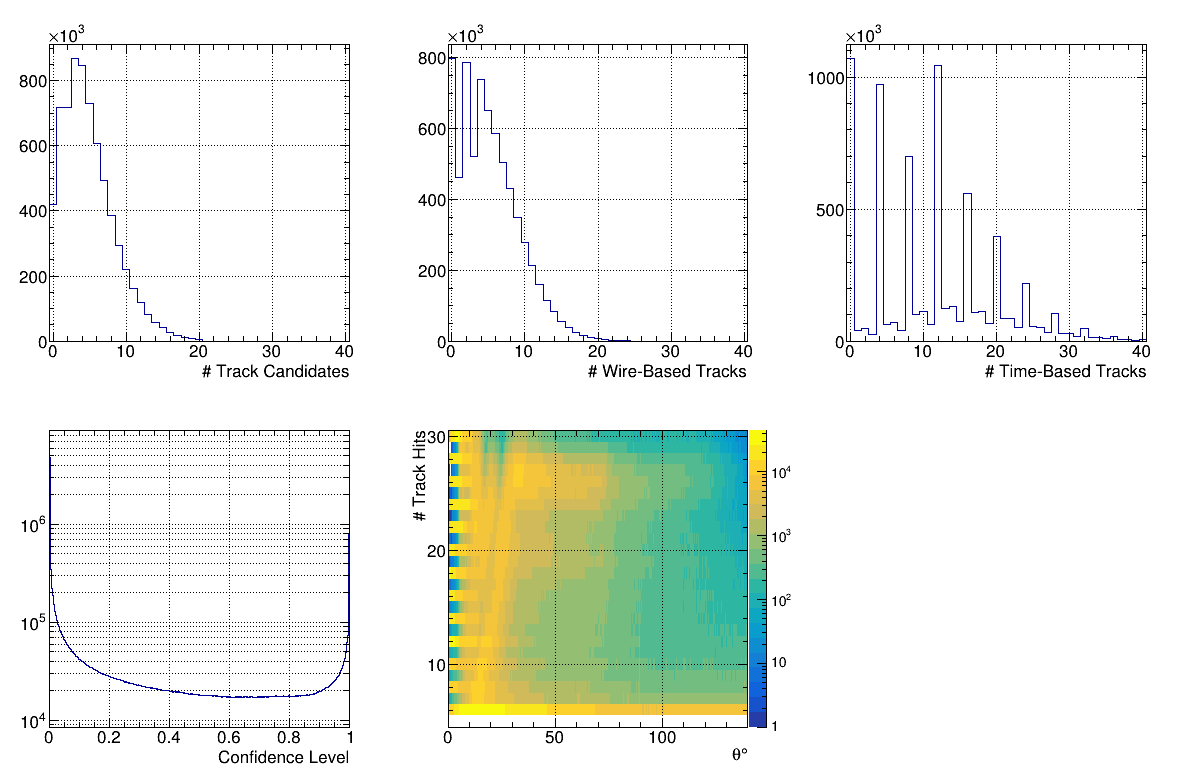
* Tracking 1 - There should be some mild dependence on beam current and radiator. Note the spikes in the upper right plot are because we have 4 hypotheses fit to a track by default. The lower left plot does have a peak at zero. | * Tracking 1 - There should be some mild dependence on beam current and radiator. Note the spikes in the upper right plot are because we have 4 hypotheses fit to a track by default. The lower left plot does have a peak at zero. | ||
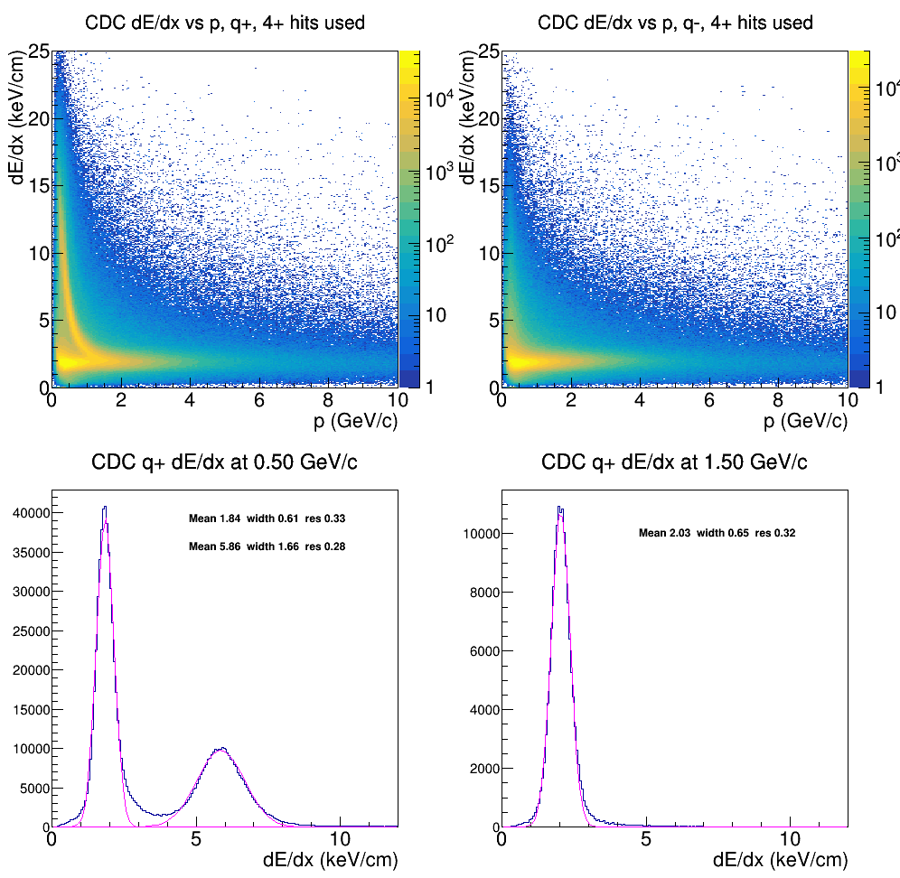
| − | * Tracking 3 - | + | * Tracking 3 - All four plot should have the pion band around 2keV/cm. Only the top left one should have an additional banana-shaped band for the protons. |
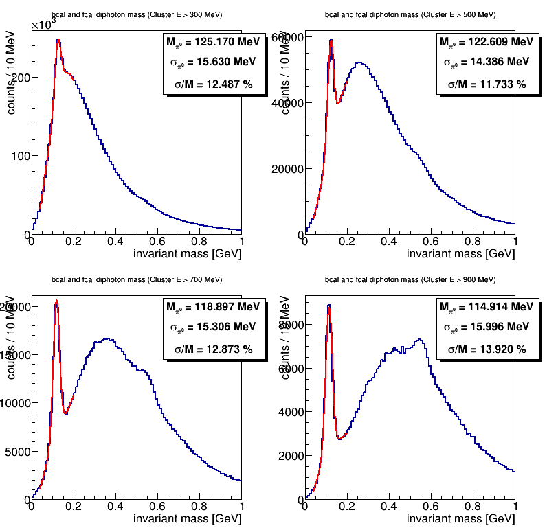
* Check BCAL pi0 - The fitted peak should near at the correct pi0 mass of 135 MeV. | * Check BCAL pi0 - The fitted peak should near at the correct pi0 mass of 135 MeV. | ||
* Check BCAL/FCAL pi0 - The fitted peak should be lower than the correct pi0 mass, I think because the wrong vertex is used. | * Check BCAL/FCAL pi0 - The fitted peak should be lower than the correct pi0 mass, I think because the wrong vertex is used. | ||
Revision as of 12:54, 28 February 2024
This page contains the procedure for checking if production runs are of good quality and can be used for physics analysis.
Contents
Run Periods
- RunPeriod-2016-02 Validation
- RunPeriod-2016-10 Validation
- RunPeriod-2017-01 Validation
- RunPeriod-2018-01 Validation
- RunPeriod-2018-08 Validation
- RunPeriod-2019-01 Validation
- RunPeriod-2019-11 Validation
- RunPeriod-2021-08 Validation
- RunPeriod-2022-05 Validation
- RunPeriod-2022-08 Validation
- RunPeriod-2023-01 Validation
Procedure
For each production run, do the following:
- Go to the Offline Run Browser page.
- Follow the steps outlined in the checklist below.
- Workers should check each plot for their assigned subsystem and leave notes in the corresponding spreadsheet if any significant deviations are seen
- On the spreadsheet, enter "Y" in the "Overall Quality" field if all monitoring histograms are acceptable, otherwise enter "N"
- We will iterate this procedure until the process converges
Expert Actions
- Certify that each subsystem is okay
- Set run status in RCDB based on monitoring results
- (script provided)
Run Statuses
- -1 - unchecked
- 0 - rejected (not physics-quality)
- 1 - approved
- 2 - approved long/"mode 8" data
- 3 - calibration / systematic studies
Checklist
Example Monitoring Spreadsheet
Reference run for 2017-01: 30780
Reference run for 2018-01: 40933/4
Reference run for 2018-08: 51388
Reference run for 2019-11: 71463 (150 nA), 71469 (250 nA), 71724 (350 nA)
Reference run for 2023-01: 120888
Expert list
Experts should update the table as tasks are completed
| Subdetector | Plots | Instructions | Expert(s) |
|---|---|---|---|
| BCAL | Good | Good | Mark Dalton, Zisis Papandreou |
| CDC | Good | Good | Naomi Jarvis |
| FCAL | ? | ? | Mark Dalton, Malte Albrecht, Igal Jaegle |
| FDC | Good | Good | Lubomir Pentchev |
| PS | ? | ? | Alex Somov, Olga Cortes |
| SC | ? | ? | Beni Zihlmann |
| TAGH | ? | ? | Alex Somov, Bo Yu |
| TAGM | ? | ? | Richard Jones, Ellie Prather |
| TOF | ? | ? | Paul Eugenio, Beni Zihlmann |
| RF | ? | ? | Sean Dobbs, Beni Zihlmann |
| Timing | ? | ? | Sean Dobbs |
| Analysis | Good | Good | Alex Austregesilo |
General Notes
- Diamond and amorphous (AMO) runs have different beam energy spectra, which leads to differences in reaction yield distributions which depend on the kinematics of the produced particles.
- The list of experts on different detector/calibration
BCAL
BCAL Reference Plots


BCAL Notes
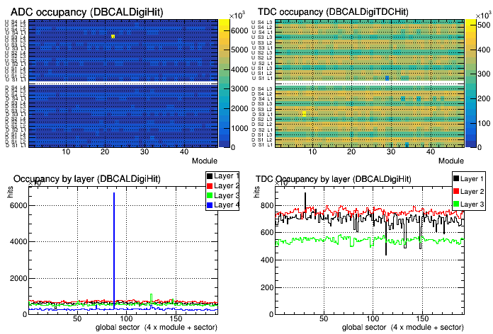
The BCAL is used to measure the energy and time of showers.
- Occupancy: This should be approximately flat. There can be hot channels when the baseline drifts.
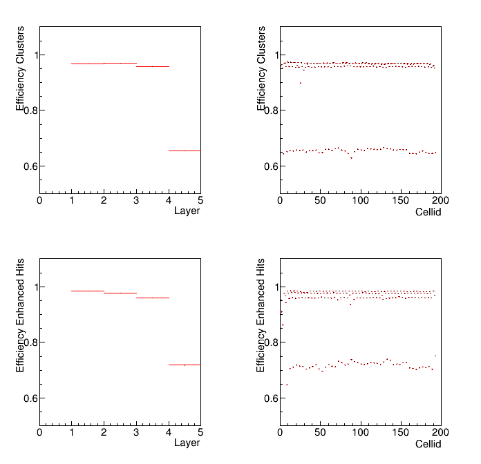
- Hit Efficiency: This should be approximately flat. If there are features we should understand why.
CDC
- Check Occupancy - Reference: [ link ]
- Check Time-to-distance - Reference: [ link ]
- Check dE/dx - Reference: [ link ]
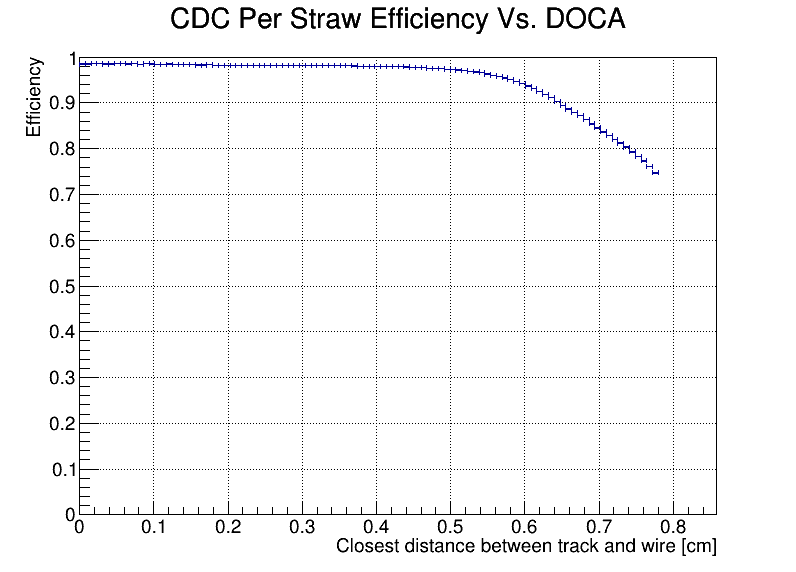
- Check Efficiency- Reference: [ link ]
CDC Reference Plots


CDC Notes
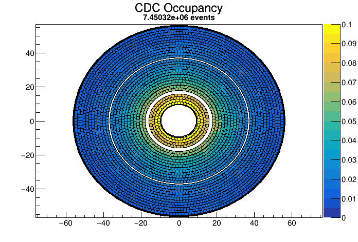
CDC Occupancy: There should be a uniform decrease in intensity from the center of the detector outward. Random white cells scattered throughout occur when not enough data were collected, eg empty target runs, trigger tests or no beam. Several contiguous white, dark blue or bright yellow cells which don't match the neighboring cells are a problem.
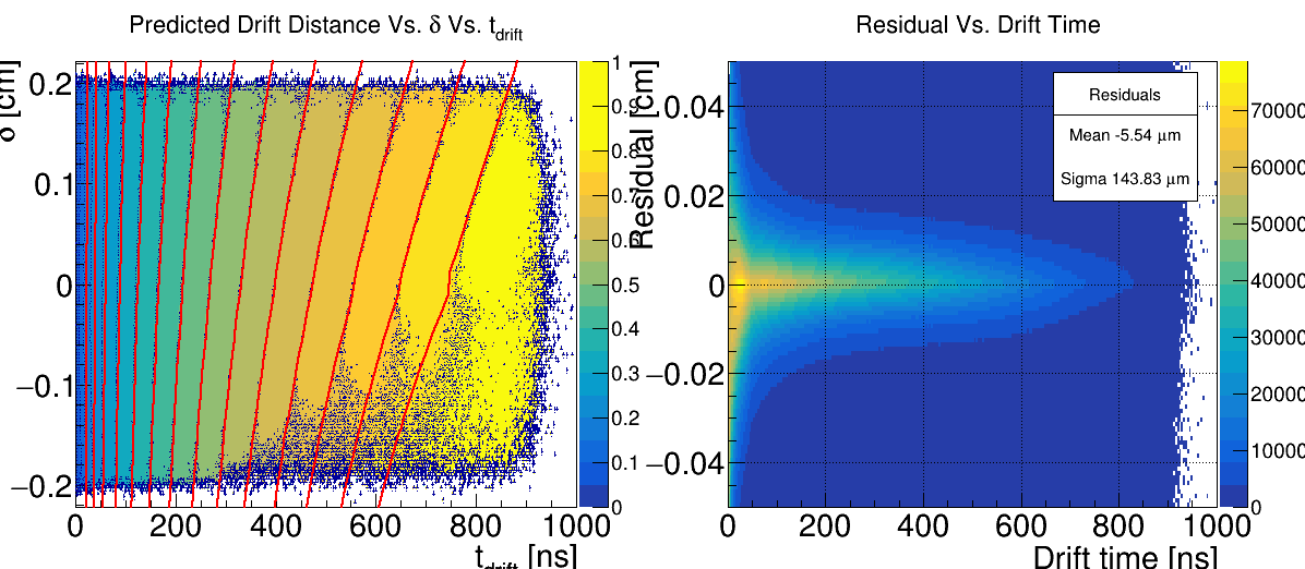
Time-to-distance: 𝛿, the change in length of the LOCA caused by the straw deformation, is
plotted against the measured drift time, t drift . The color scale indicates the distance of
closest approach between the track and the wire, obtained from the tracking software.
The red lines are contours of the time-to-distance function for constant drift distances
from 1.5 mm to 8 mm, in steps of 0.5 mm. They should lie over the top of the dark blue contour lines separating the colour blocks.
For the plot of residuals vs drift time, the mean should be less than 15um and the sigma should be less than 150um.
dE/dx: At 1.5GeV/c the fitted peak mean should be within 1% of 2.02 keV/cm.
Efficiency: The efficiency should be 0.98 or higher at 0cm DOCA, gradually fall to 0.97 at approximately 0.5mm and then more steeply through 0.9 at approximately 0.64cm.
FCAL
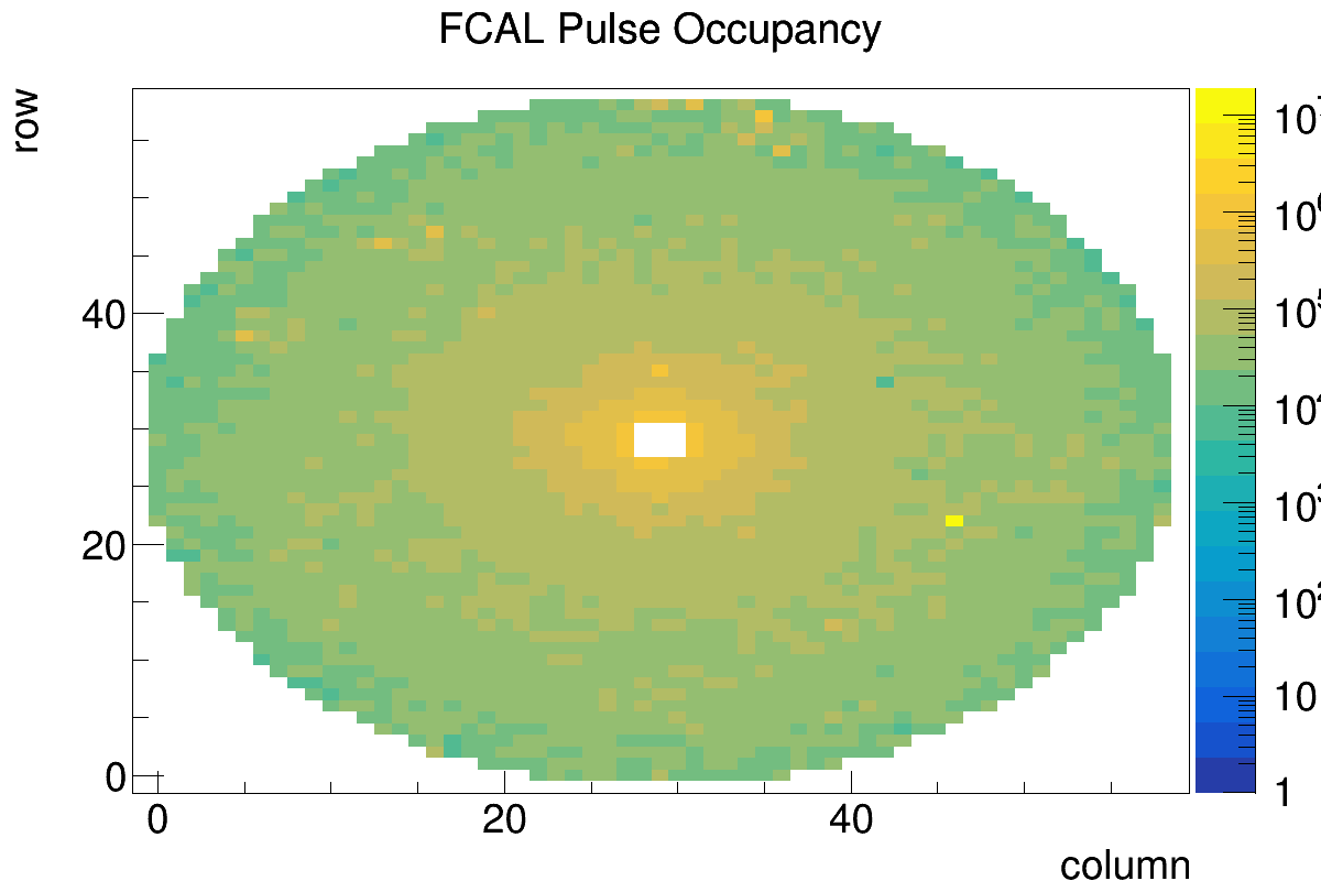
- Check Occupancy - Reference: [ link ]
FCAL Reference Plots

FCAL Notes
Is used for neutral particle detection and pion identification.
- Check Occupancy:
FDC
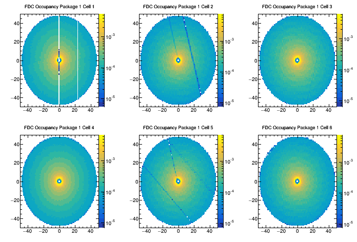
- Check Package 1 Occupancy - Reference: [ link ]
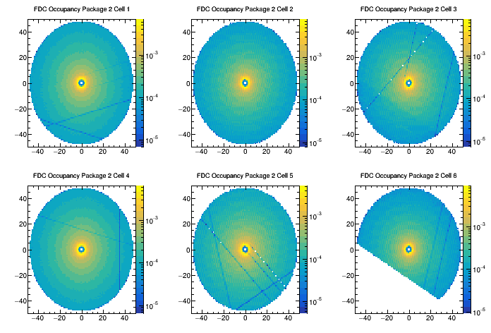
- Check Package 2 Occupancy - Reference: [ link ]
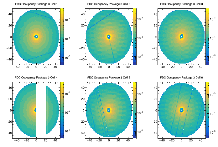
- Check Package 3 Occupancy - Reference: [ link ]
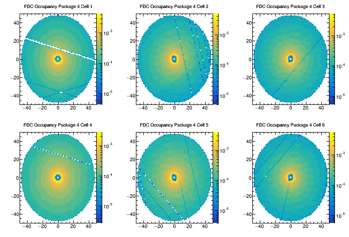
- Check Package 4 Occupancy - Reference: [ link ]
FDC Reference Plots


FDC Notes
There are two HV sectors, in Package 2 cell 6 (28 wires) and Package 3 cell 4 (20 wires), that are always OFF and seen in the occupancy plots as empty sectors. There are also strips with lower or no efficiency that are always there, mostly in Package 3 and 4 (see the reference plots), which also normal. What is not normal are groups of wires (of the order of 8 to 24 wires) that are noisy. They will show as brighter stripes in the occupancy. The problem is that they may lock the F1TDCs. This happened several times in the past years. In general, look for groups of channels that are overactive or have lower efficiency.
The reference plots show pseudohits, generated from the track reconstruction. If you find an abnormality, it would be helpful to check 2 more histograms to find the underlying cause - 'FDC Hit Occupancy' will show if any channels are missing, and 'HLDT Drift Chamber Timing' (bottom right plot) will show TDC time-shifts.
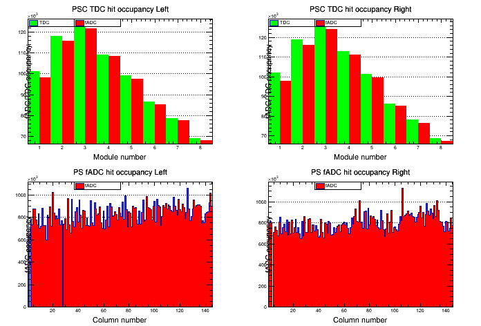
PS
PS Reference Plots


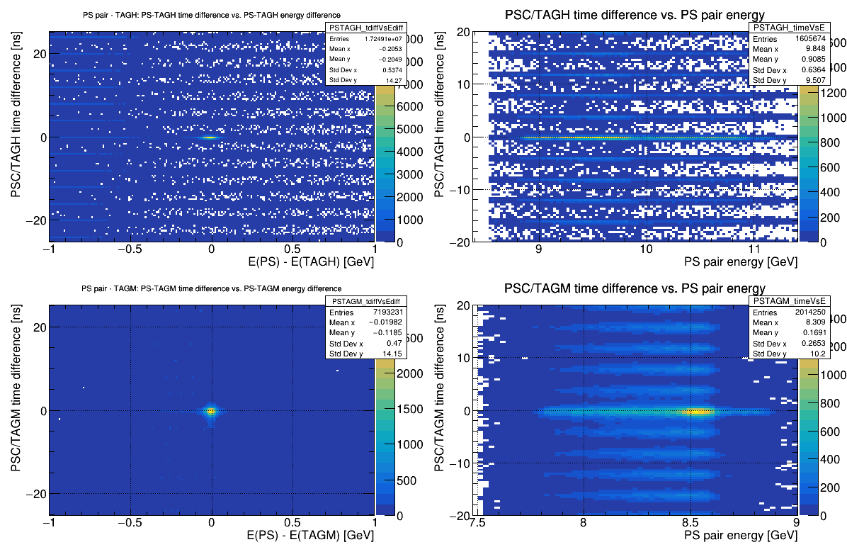
PS Notes
SC
- Check Occupancy - Reference: [ link ]
- Check Recon. SC 1 - Reference: [ link ]
- Check Recon. SC 2 - Reference: [ link ]
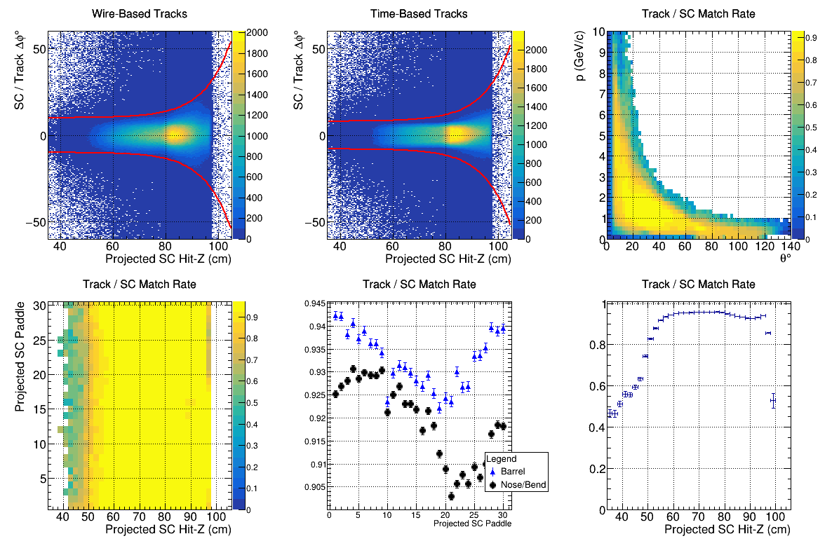
- Check Recon. SC Matching - Reference: [ link ]
SC Reference Plots


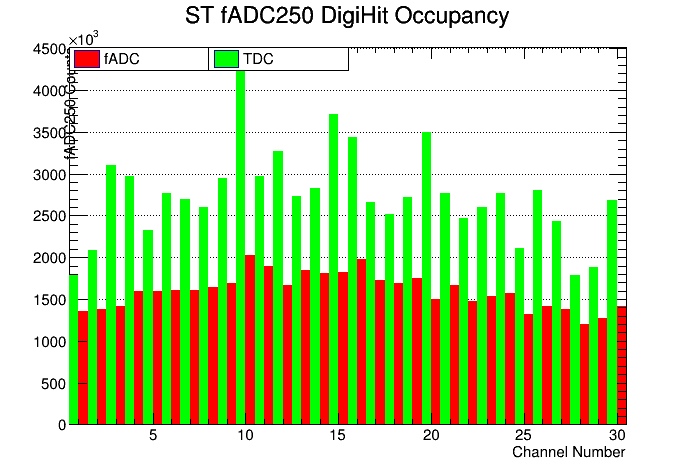
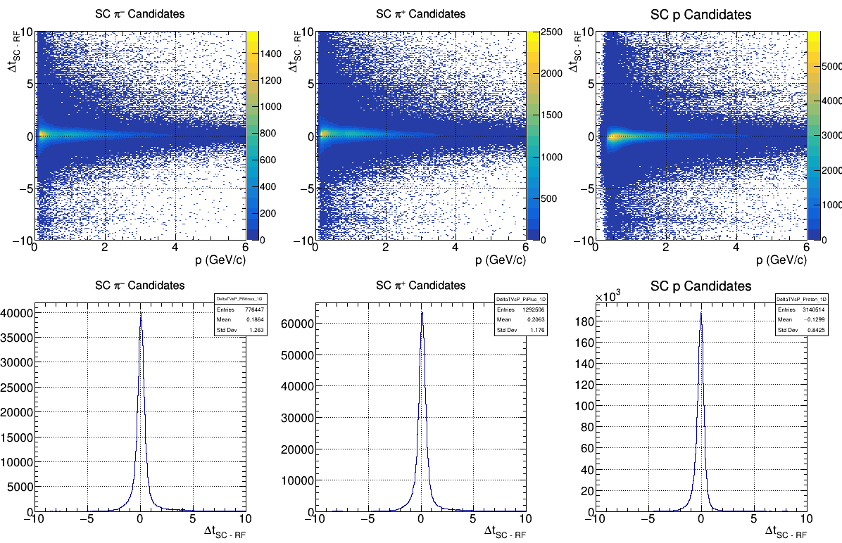
SC Notes
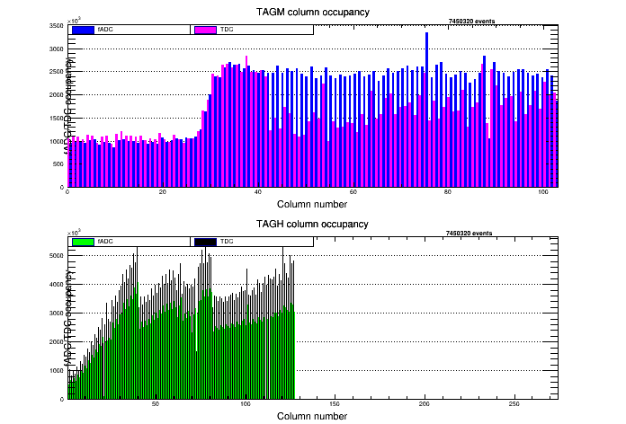
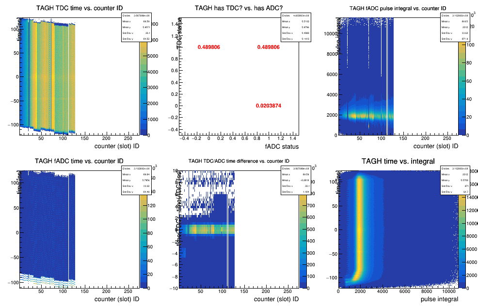
TAGH
TAGH Reference Plots


TAGH Notes
TAGM
TAGM Reference Plots


TAGM Notes
TOF
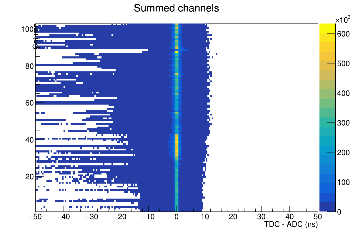
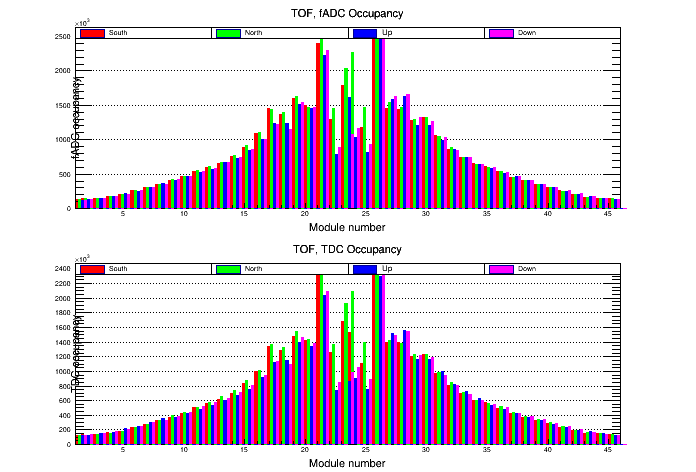
- Check Occupancy - Reference: [ link ]
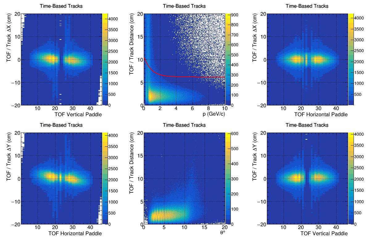
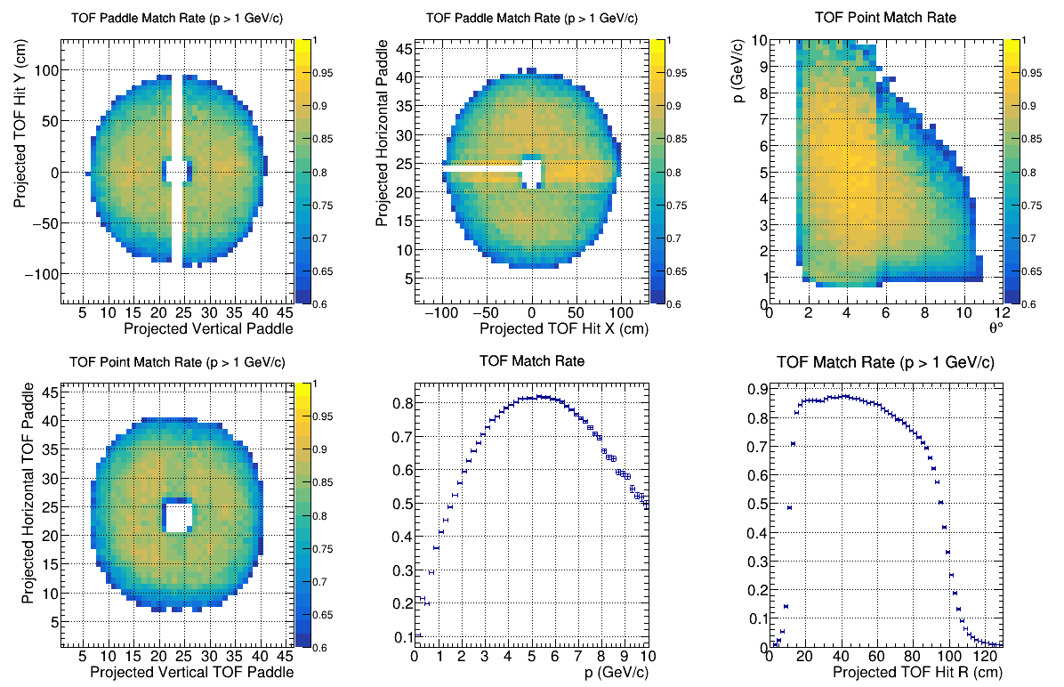
- Check TOF Matching 1 - Reference: [ link ]
- Check TOF Matching 2 - Reference: [ link ]
TOF Reference Plots


TOF Notes
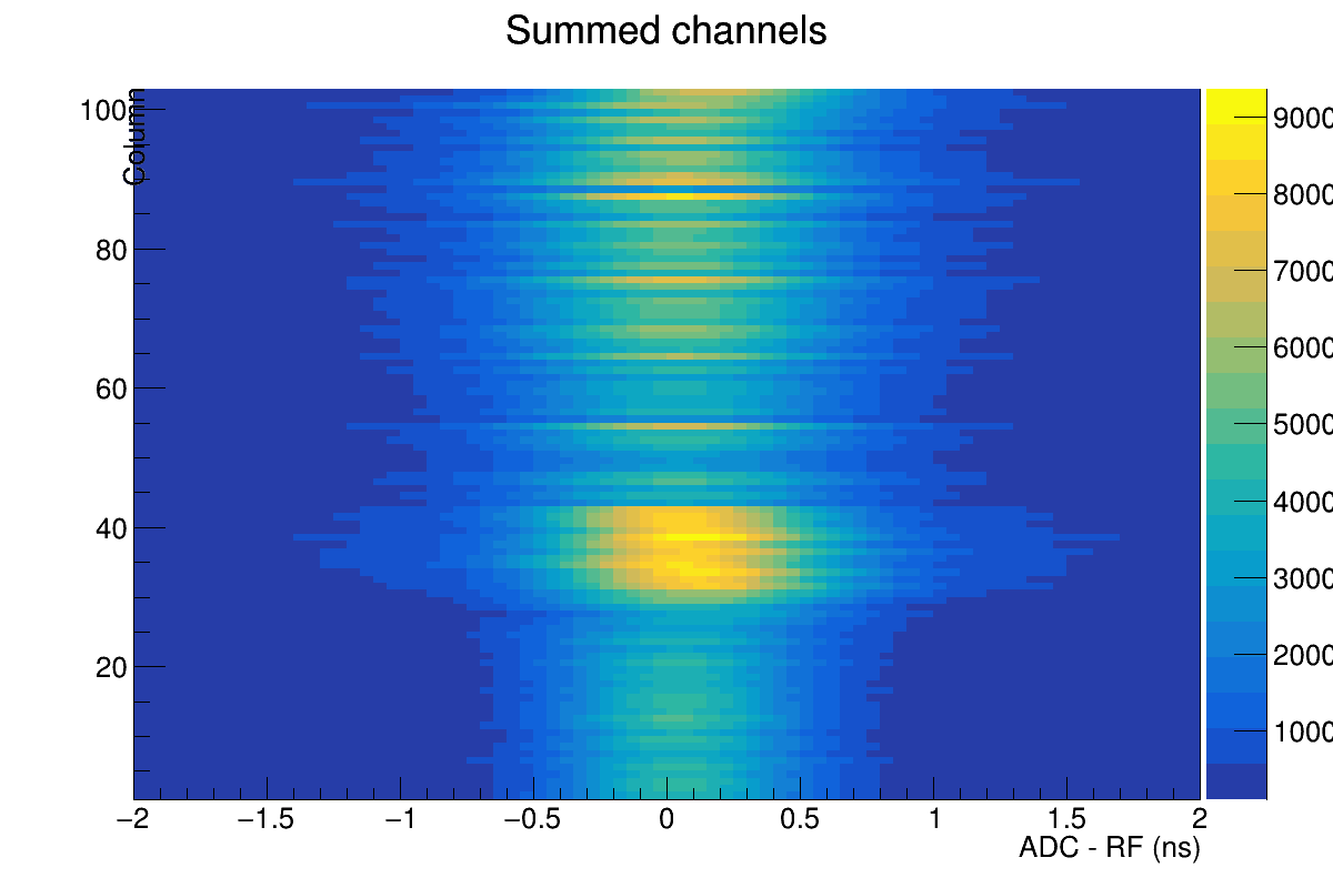
RF
- Check timing offsets - Reference: [ link ]
- Should be centered around zero
RF Reference Plots

Timing
- Check HLDT Calorimeter Timing - Reference: [ link ]
- Check HLDT Drift Chamber Timing - Reference: [ link ]
- Check HLDT PID System Timing - Reference: [ link ]
- Check HLDT Tagger Timing - Reference: [ link ]
- Check HLDT Tagger/RF Align 2 - Reference: [ link ]
- Check HLDT Tagger/SC Align - Reference: [ link ]
- Check HLDT Track-Matched Timing - Reference: [ link ]
Timing Reference Plots

![]()


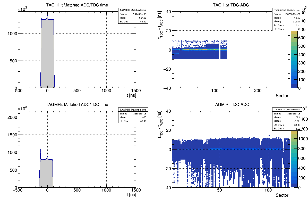
Timing Notes
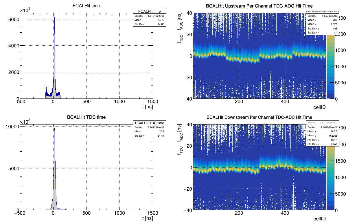
- Calorimeter Timing - The right two plots aren't aligned at zero because not all corrections are currently applied. If there is a 32 ns shift in part of this data, please note this.
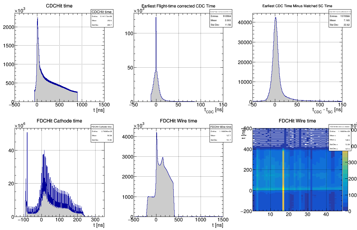
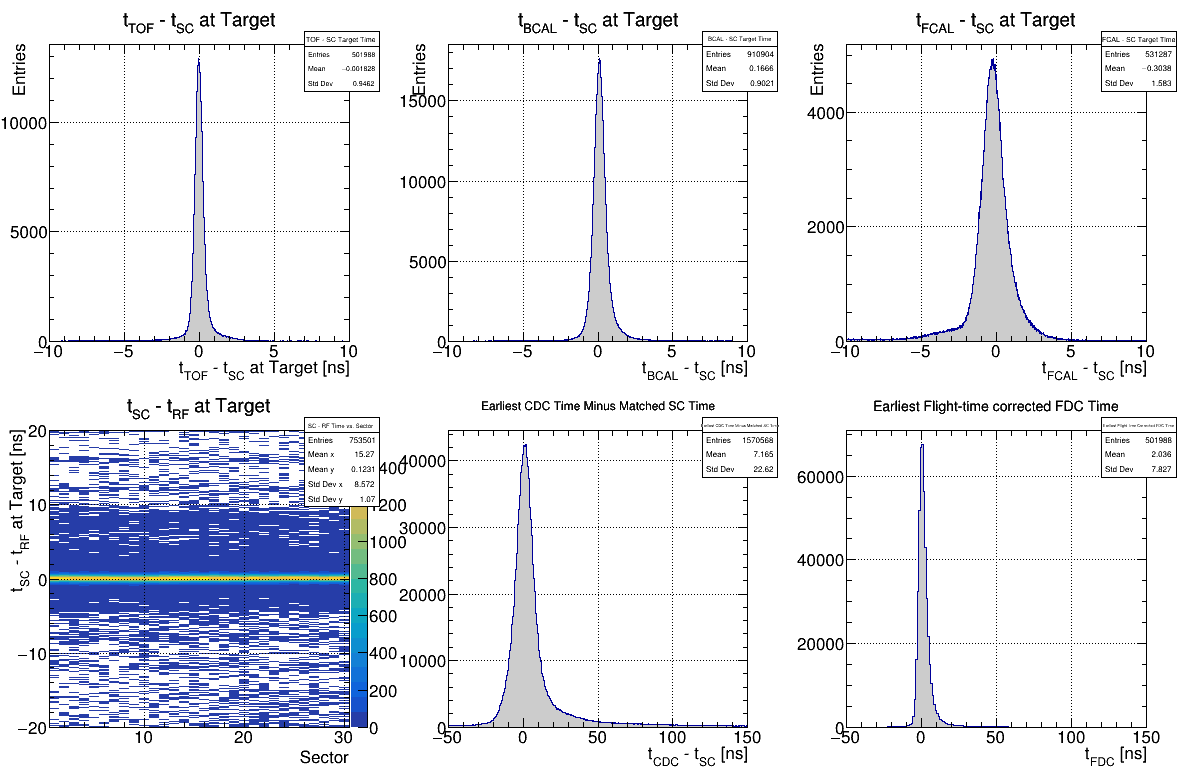
- Drift Chamber Timing - In each case, the main peaks should line up at zero, but often have other structures. Ignore the first few bins of the lower left plot (they mostly say something about the noise in the detector). There can be 32 ns shifts in the lower right plot.
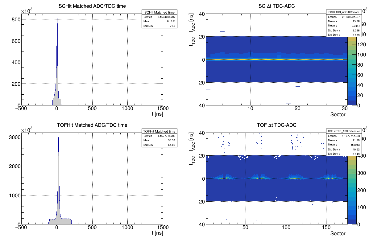
- PID System Timing - Nothing to note yet.
- Tagger Timing - The signal to background levels of the left two plots depend on the electron beam current.
- Track Matched Timing - Some overlap here with the tracking timing. The new plots should be centered at zero.
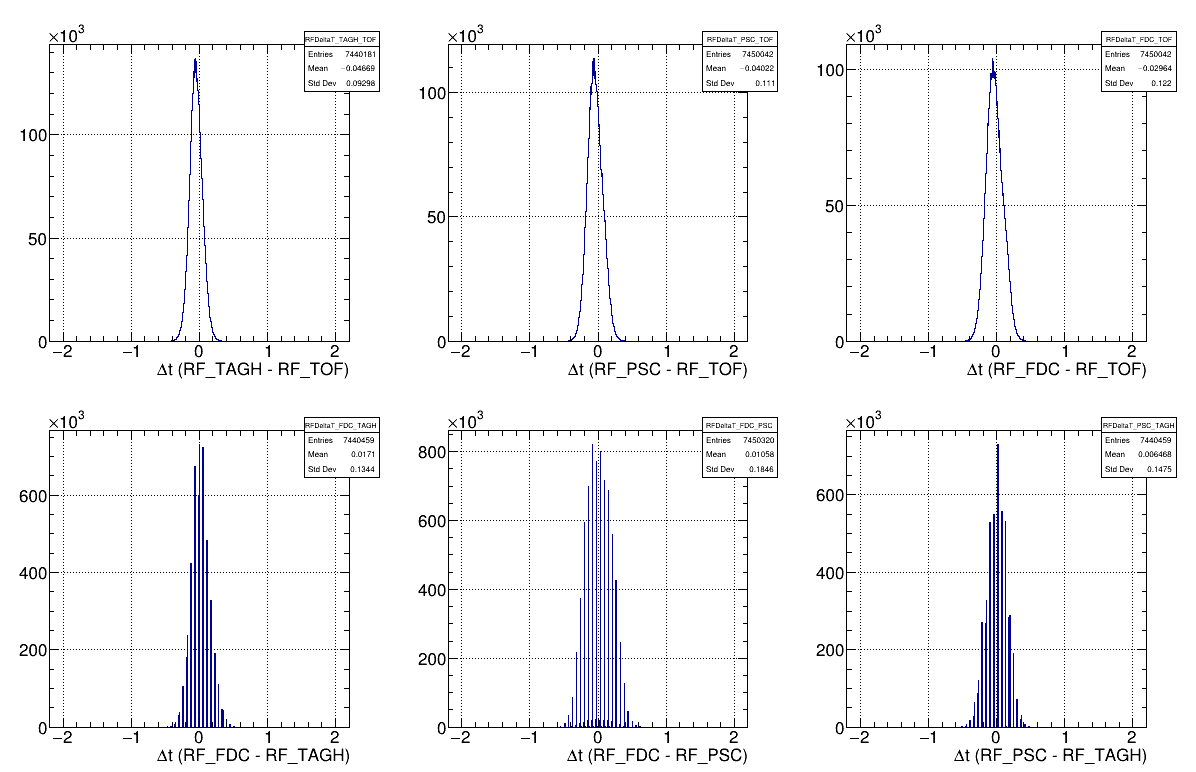
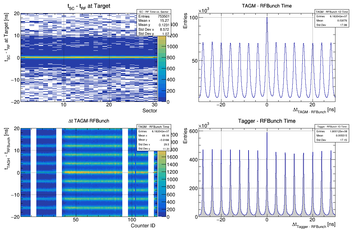
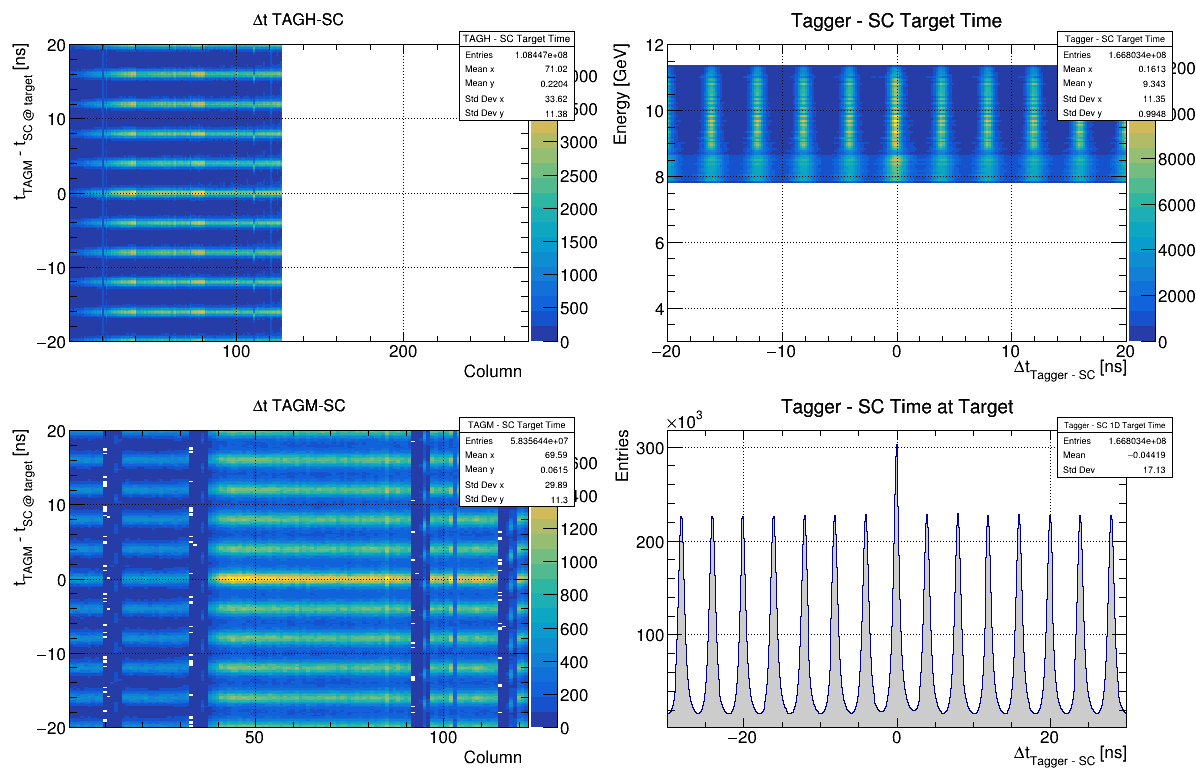
- Tagger/RF Timing - Look for the nice "picket fences" on the right two plots, and that in the bottom left plot each channel peaks at zero.
- Tagger/SC Timing - Should be similar to Tagger/RF Timing but with larger resolution.
Analysis
- Tracking 1 - [ link ]
- Tracking 3 - [ link ]
- Check BCAL pi0 - Reference: [ link ]
- Check BCAL/FCAL pi0 - Reference: [ link ]
- Check p+2pi - Reference: [ link ]
- Check p+3pi - Reference: [ link ]
- Check p+pi0g - Reference: [ link ]
Analysis Reference Plots
![]()
![]()


Analysis Notes
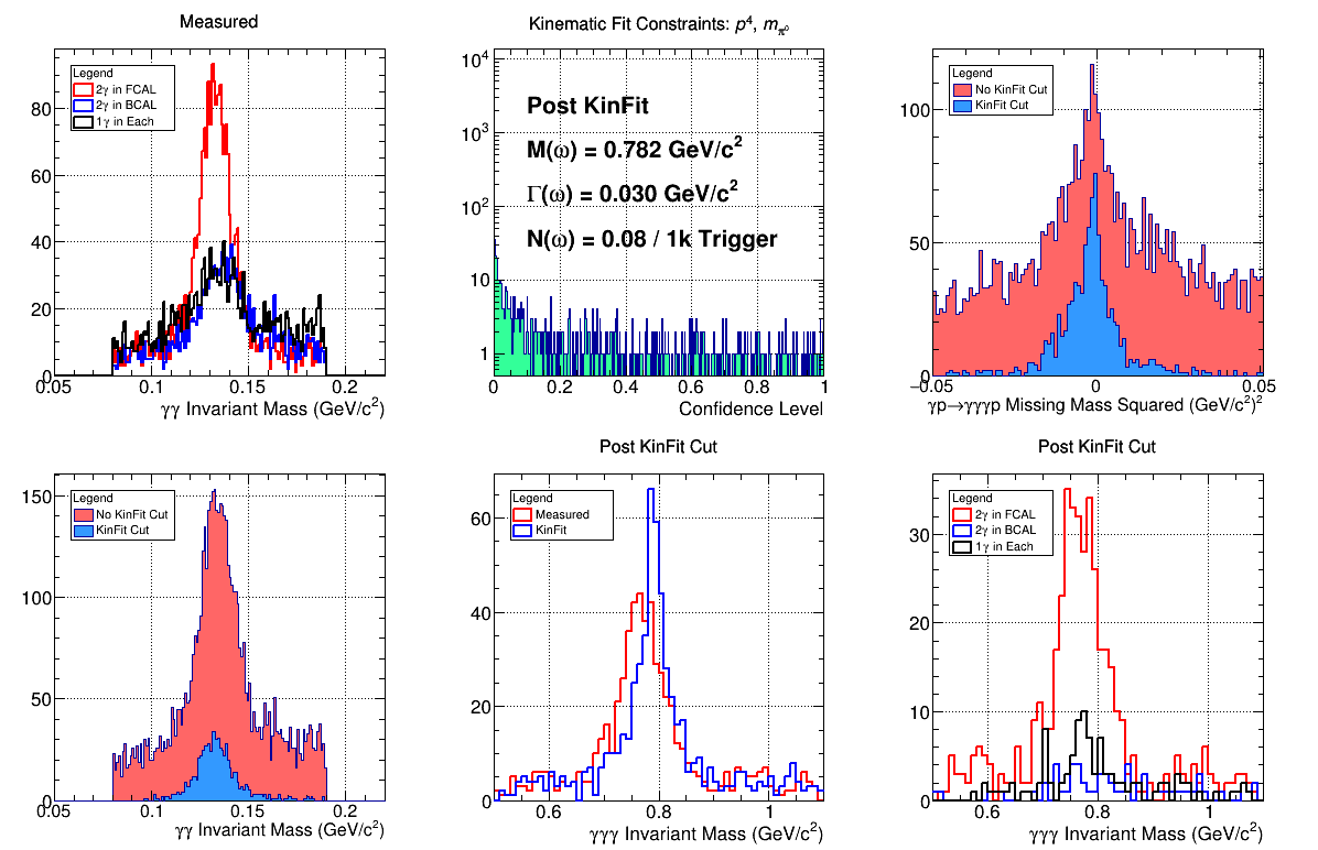
Generally in these plots, there will be a difference between diamond and amorphous radiator running. Should probably add some references for non-diamond plots.
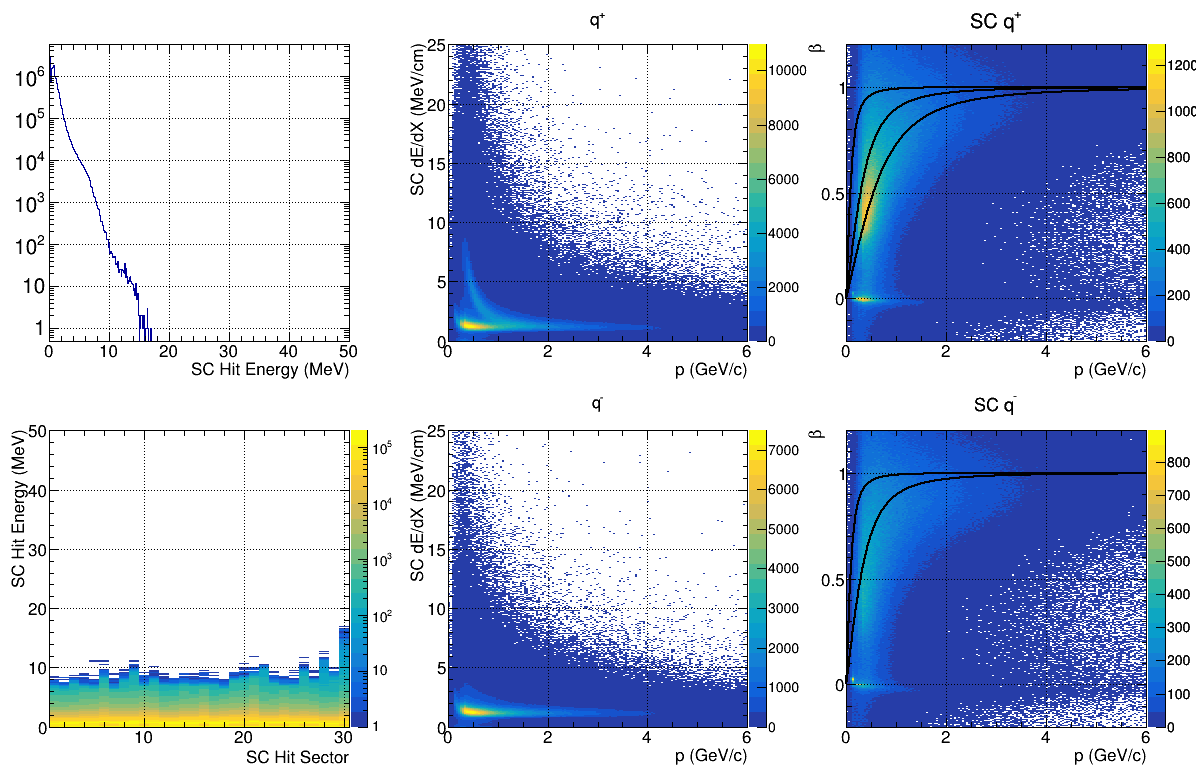
- Tracking 1 - There should be some mild dependence on beam current and radiator. Note the spikes in the upper right plot are because we have 4 hypotheses fit to a track by default. The lower left plot does have a peak at zero.
- Tracking 3 - All four plot should have the pion band around 2keV/cm. Only the top left one should have an additional banana-shaped band for the protons.
- Check BCAL pi0 - The fitted peak should near at the correct pi0 mass of 135 MeV.
- Check BCAL/FCAL pi0 - The fitted peak should be lower than the correct pi0 mass, I think because the wrong vertex is used.
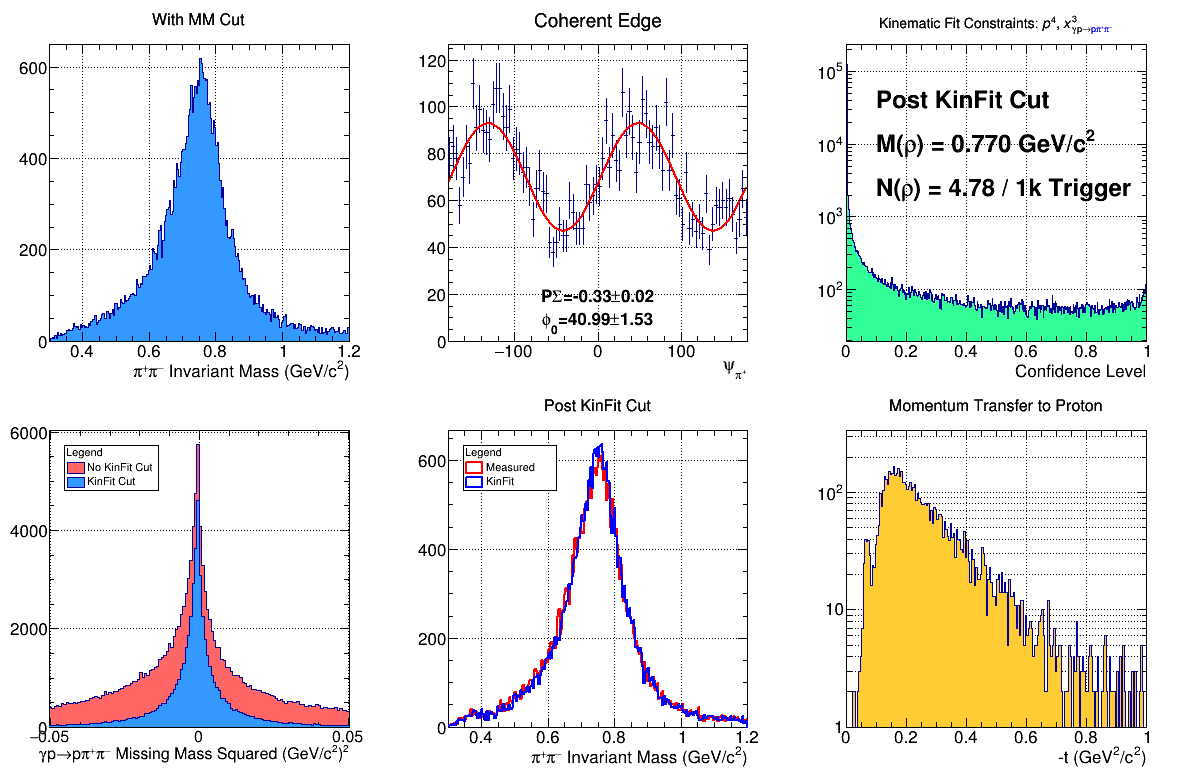
- Check p+2pi - The top middle plot should have a sin(2phi) shape for diamond runs. Note that the yields in the top right plot vary from run to run on the order of 10-20%.
- Check p+3pi -Note that the yields in the top right plot vary from run to run on the order of 10-20%.
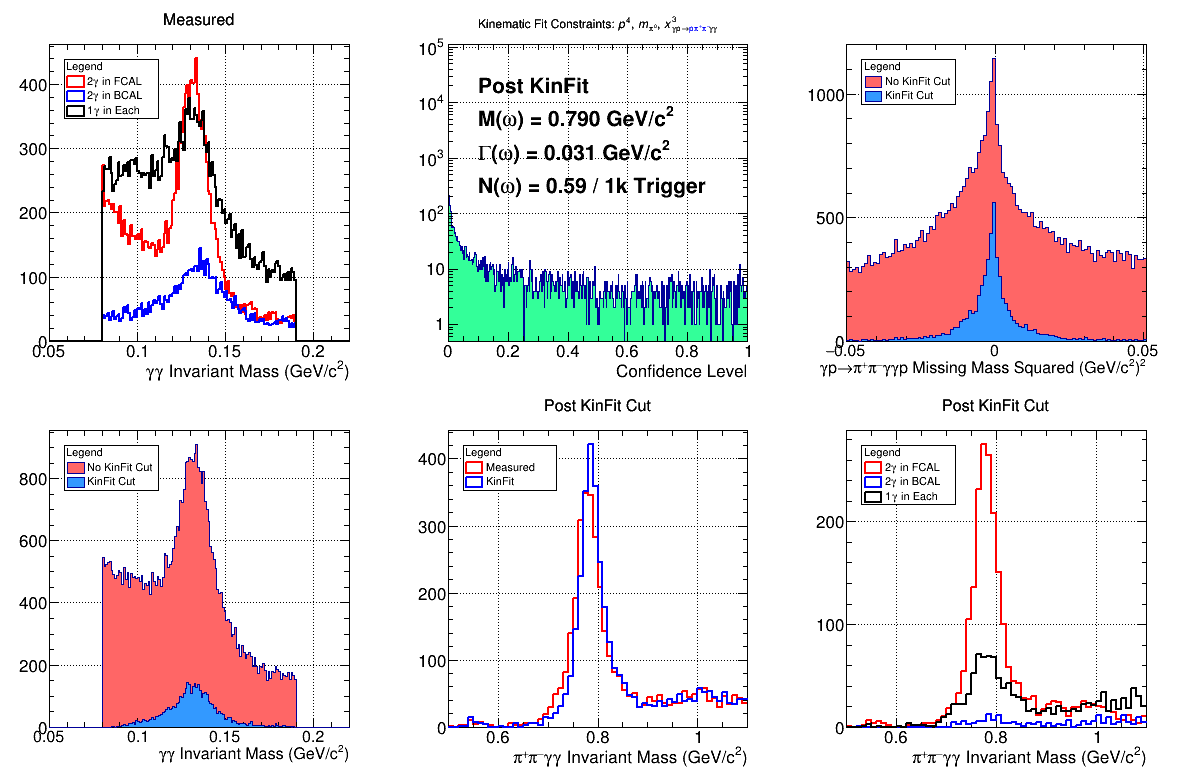
- Check p+pi0g - Note that the yields in the top right plot vary from run to run on the order of 10-20%.
- Note that these yields are sensitive to the tagger range used! This changes for different beam current settings.